Introduction
Modern CPUs have a clock speed measured in gigahertz, a far cry from the original kilohertz speeds of the first CPUs. However, the workloads we place upon these chips have also vastly grown. Because of this, anyone who writes code needs to contend with the efficiency of their programs. Well-optimized code ensures that your program can handle today’s modern computing tasks, whether it be working with big data sets, time-sensitive applications, or running on low-power hardware. Conversely, a poorly optimized program can needlessly slow down execution, leading to sluggish performance and at worst, failure of critical components. Therefore, the ability to analyze your code and make the necessary optimizations is imperative to creating efficient and usable applications.
The first step in optimization is often to simply find the execution time of your code. Without which, how would one know if changes are actually improving the time efficiency of your program? Here, we’ll develop a reusable Python function that allows us to measure the average time it takes another function to run. While there are several Python libraries that have timing capabilities, I have found that it is difficult to find one that allows for the easy timing of complex functions with many parameters. I encourage to research these other libraries on your own, as many offer a convenient solution for simple timing tasks. However, by the end of this tutorial, we’ll have a more robust timing solution that can easily be applied to most of your Python functions.
Python Function Timer
To build our function timer, we’ll rely on Python’s time module, which provides an interface to several time related functions. In particular, we’ll use time.perf_counter function. This returns a float value from a performance counter in seconds. However, it is important to note that the reference point of the counter is undefined. That is, the counter does not start at zero, but at some arbitrary value. Therefore, we calculate the time by caching the value of the counter before and after the code we want to time and calculating the difference:

Using this method, we can get the execution time of any code as follows:
Code Listing 1: Using Python’s Time Module to Get Execution Time
import time

# Get start time
startTime = time.perf_counter()

# Code block that you want to time
numList = []
for i in range(100000):
  numList.append(i)

# Get end time
endTime = time.perf_counter()

# Calculate and display total time
totalTime = endTime - startTime
print("Total Time: " + str(totalTime) + " (s)")
Output:
Total Time: 0.02836027000012109 (s)
Here, we simply got the execution time of making a list of numbers, but you could use this method to find the execution time of any block of code. However, there is a problem with this implementation. If you run this code many time, you’ll notice that the time will fluctuate, sometimes quite dramatically. This is because at any given moment, your processor is juggling many different tasks and its scheduler is dynamically priortizing these tasks and allocating resources. Therefore, the execution time of your python code at runtime is dependent on the current state of your system and its background tasks. To account for this, instead of timing a single run of the code, it is more representative to calculate the average execuation time. This can be easily accomplished by iterating over the code your want to time:
Code Listing 2: Calculating the Average Execution Time Using Multiple Iterations
import time

# Set the number of iterations to run the code block
numIterations = 100

# Initialize the time sum to zero
timeSum = 0

# Iterate the code block
for _ in range(numIterations):
  # Get the start time
  startTime = time.perf_counter()
  # Code block that we want to time
  numList = []
  for i in range(100000):
    numList.append(i)

  # Get the end time
  endTime = time.perf_counter()
  # Add the execution time to the running sum
  timeSum += endTime - startTime

# Caclulate the average execution time and display results
avgTime = timeSum/numIterations
print("Average Time: " + str(avgTime) + " (s)")
Output:
Average Time: 0.012075293239940948 (s)
The above is suitable if you only need to time a small block of code. However, I often find myself needing to time larger functions. Therefore, let’s finally build our timeing function. For this, we can use the foundations we have covered to build a timing function that will allow us to find the average execution time of other python functions:
Code Listing 3: Timer Function
import time

def time_function(func, numIterations, *args, **kwargs):
  timeSum = 0
  for _ in range(numIterations):
      startTime = time.perf_counter()
      func(*args, **kwargs)
      timeSum += time.perf_counter() - startTime
  avgTime = timeSum/numIterations
  return avgTime
We start by defining our time_function. As parameters, we take in another python function, func, as the function we want to find the execution time of. We then set the number of iterations, numIterations, that we want to run the function over to find the average time. If the function, func, requires its own parameters, we can pass those in using *args and *kwargs. From there, the function operates in a similar manner to our previous timing examples. The only difference being that instead of timing a code block, we call the function we want to time upon each iteration. Lastly, our timing function will return a float representing the average execution time of the function.
Example Implementation
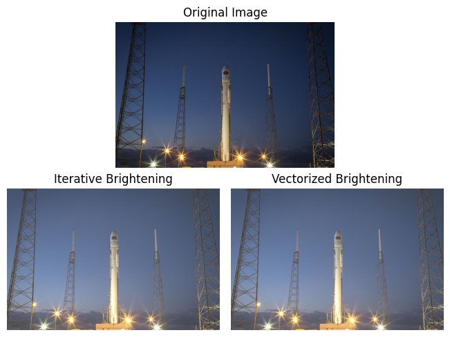
Here, let’s examine how to implement our python timer function. As an example, let’s say we are trying to write a function that will allow us to brighten an image. As some quick background, images can be represented as arrays or pixels values, and image brightening can be achieved by simply adding a constant each pixel. We’ll write two different image brightening functions, one in which we iterate through each pixel value and another where we take advantage of numpy’s vectorization. We expect the vectorized implementation to be much faster and we’ll use our timing function to calculate the speedup:
Code Listing 4: Timing Example Image Brightening Functions
import time
import numpy as np
import skimage as sk
import matplotlib.pyplot as plt
import matplotlib.gridspec as gridspec

# Get an example image from sci-kit image
img = sk.data.rocket()

# Iterative brightening function
def brighten_img_iterative(img, offset, rgb=False):
  ''' Loops through x, y (and z if rgb) dimensions of image and adds an
  offset to each pixel value. Checks if offset will make pixel exceed 255
  allowed for 8bit images, and if so, sets pixel value to 255. '''
  output = np.zeros(img.shape)
  if not rgb:
    for i in range(img.shape[0]):
      for j in range(img.shape[1]):
        if img[i,j] + offset > 255:
          output[i,j] = 255
        else:
          output[i,j] = img[i,j] + offset
  else:
    for i in range(img.shape[0]):
      for j in range(img.shape[1]):
        for k in range(img.shape[2]):
          if img[i,j,k] + offset > 255:
            output[i,j,k] = 255
          else:
            output[i,j,k] = img[i,j,k] + offset
  return output.astype(np.uint8)

# Vectorized brightening function
def brighten_img_vectorized(img, offset):
  '''Casts image to uint32 to avoid rollover when adding offset to array.
  Sets all values greater than 255 to 255, and recasts back to unint8'''
  img = img.astype(np.uint32)
  output = img + offset
  output[output > 255] = 255
  return output.astype(np.uint8)

# Get average execution time of both iterative and vectorized methods
iterativeTime = time_function(brighten_img_iterative, 10, img, 50, rgb=True)
vectorizedTime = time_function(brighten_img_vectorized, 10, img, 50)

# Calculate speedup acheived with the vectorized method
speedUp = iterativeTime/vectorizedTime

# Display results the console
print("Iterative Time: " + str(iterativeTime) + " (s)")
print("Vectorized Time: " + str(vectorizedTime) + " (s)")
print("Speed Up: " + str(speedUp))

# Get brightened images using both methods
imgBrightIter = brighten_img_iterative(img, 50, rgb=True)
imgBrightVec = brighten_img_vectorized(img, 50)

# Configure matplotlib subplot
imgFig = plt.figure(constrained_layout=True)
spec = gridspec.GridSpec(ncols=2, nrows=2, figure=imgFig)
ax1 = imgFig.add_subplot(spec[0, :])
ax2 = imgFig.add_subplot(spec[1, 0])
ax3 = imgFig.add_subplot(spec[1, 1])

# Plot the resultant images
ax1.imshow(img)
ax1.set_title("Original Image")
ax1.axis("off")
ax2.imshow(imgBrightIter)
ax2.set_title("Iterative Brightening")
ax2.axis("off")
ax3.imshow(imgBrightVec)
ax3.set_title("Vectorized Brightening")
ax3.axis("off")
plt.show()
Output:
Iterative Time: 6.3284335391 (s)
Vectorized Time: 0.0015949406999993699 (s)
Speed Up: 3967.817448700444
In the above code, we define our two brightening functions, brighten_img_iterative and brighten_img_vectorized. Then, on the highlighted lines, we use our timing function to calculate the average execution time of each brightening method. It is important to note the parameter layout of our timing function: time_funtion(func, numIterations, *args, *kwargs). Remember that numIterations is the number of iterations to find the average time, and that *args and *kwargs are the parameters of func. To show this more clearly, consider the line of code in which we find the average execution time of the iterative brightening function:
iterativeTime = time_function(brighten_img_iterative, 10, img, 50, rgb=True)
Here, I have color-coded to show the relationship between the different parameters. In this case, iterativeTime is a float representing the average execution time as calculated by timing 10 iterations of function calls to brighten_img_iterative(img, 50, rgb=True).
Examining the output of our example code, we see that the vectorized implementation of image brightening is indeed substantially faster that the iterative approach. In fact, it is nearly 4000 times faster, while yielding an identical result. This is due to numpy’s memory optimization, parallel computation, and it’s C language implementation, all of which contribute to its efficiency.
Wall-Clock Time vs. CPU Time
Thus far, the times we have calculated have been wall-clock times (also known as elaspsed real time). That is, the time returned from our timer is the actual amount of time elapsed between the start and end of our function. As mentioned previously, this can include waiting for resources, input/output, and other tasks to finish. However, we can also measure the cpu time, which only accounts for the time that the cpu is actively working on your program. We can quickly modify our timer function to instead calculate cpu time by using time.process_time, instead of time.perf_counter. The method time.process_time returns a float representing the sum of the system and user cpu time. Like the performance counter, time.process_time is unreferenced, meaning that you still need to calculate the difference between two subsequent calls for the time:
Code Listing 5: Timer Function Modified for CPU Time
import time

def time_function_cpu(func, numIterations, *args, **kwargs):
  timeSum = 0
  for _ in range(numIterations):
      startTime = time.process_time()
      func(*args, **kwargs)
      timeSum += time.process_time() - startTime
  avgTime = timeSum/numIterations
  return avgTime
Final Thoughts
As we have shown, different code implementations can achieve the same result with drastically different performance. In our example, vectorization with numpy exhibited a nearly four thousand fold increase in performance over an itertative approach. While having a solid foundation in programming principles can help you identify possible inefficient code, many times you simply need to time your implementations. Here, we have developed a reusable timing function to help you determine the execution time of your code. From there, you have a baseline from which you can further optimize. Ultimately, the ability to accurately measure and refine your code’s execution time will elevate your programming, leading to faster, more reliable, and efficient solutions.