
Introduction
While aspects of artificial intelligence (AI) have long been incorporated into the products and algorithms with which we interact everyday, the technology has now been thrust into the public spotlight. Propelled by recent advancements, a robust conversation has emerged around AI regarding its transformative potential and possible negative ramifications. Regardless, it is clear that this technology will continue to become more tightly integrated into our lives. Undoubtedly, many will seek to use these novel and complex AI techniques in a variety of applications. However, amid these powerful new methods, it can be all to easy to overlook more foundational techniques. In particular, it is important to recognize that some applications do not require the complexities incurred by advanced machine learning methods. In many cases, more elemental techniques can yield similar or better results, while being much easier to implement. Therefore, it is essential that while we consider these powerful AI tools, we do not overlook the fact that more rudimentary methods still may be the optimal approach to certain problems.
Here, we’ll explore Bayesian classification, one of the most foundational techniques in machine learning. In this method, we seek to use the underlying statistics of the data to form a probabilistic model for classification. When stated this way, Bayesian classification may seem complicated, however, we’ll soon see that this technique is quite intuitive and under certain circumstances, can yield optimal classification decisions. Bayesian decision theory and many of the topics covered here are widely considered the basis of pattern recognition and are indispensable to anyone in the field of machine learning.
Classification Problems
Before delving into Bayesian decision theory, let’s develop a basic understanding of classification problems, as well as form a possible mathematical framework to help us approach such problems. Broadly speaking, a classification problem is a type of problem in which a set of observations are used to make some sort of prediction about the source of the observations. This prediction is categorical, that is, given some observational data, we seek to develop a model such that we can determine the category that gave rise to those specific observations.
To clarify this, lets look at an example of a classification problem that we’ll use throughout this article. Suppose that we are tasked by a supermarket to develop a system that automatically determines what type of fruit is placed on the self checkout register. For simplicity, lets say that we only have differentiate between green apples, oranges, and grapefruit. How can we design a system and algorithm to achieve this?
A good starting point is to examine how us humans discriminate between these fruit. This starts with us making observations about the fruit. We note a bunch of information about the fruit, aspects such as its color, texture, size, shape, weight, among many others. Over the course of our lives and our repeated exposures to different kinds of fruit, our brains have developed a mental model for differentiating between the fruits. Subconsciously, our observations about the fruit are evaluated by this mental model, which allows us to recognize which fruit we are looking at. Here we can see the three main components of the classification process, the observation, model, and determined category.
To develop a method to allow a computer to perform this fruit classification, lets establish a mathematical and algorithmic definition for this process. First, we must choose a set of observations to make about the fruit. Formally, each observation is known as a feature, and the set of observations is mathematically denoted as the feature vector:
(1) 
Here,  is the feature vector, containing a
  number of individual features,
  to
to  . In our case, let’s choose the fruit’s color and weight as our features. Please note, the selection of good features is crucial to obtaining optimal classification. The process of selecting good features and extracting those features is an entire sub-problem in classification, and much is beyond the scope of this article. For now, just known that in general we want to choose features in which the categories will differ considerably. For example, when classifying between oranges and grapefruit, color is quite a non-informative feature, as the skins of oranges and grapefruits are similarly colored. However, since grapefruits are generally considerably larger than oranges, we can use the fruit weight as a better (more differentiating) feature. Lastly, the features need to actually be measured, a process known as feature extraction. This usually includes the use of sensors and preprocessing techniques to yield the actual measurement of the feature. In our example, we might use an integrated camera and scale in the self checkout machine to obtain values for our color and weight features, respectively.
A model is needed that takes the feature vector as input, and based on the features, decides the output category. Developing this model is the fundamental obstacle in classification problems. The model can be thought of as a mapping between the feature vector and the decided category. Note that there are myriad different model structures, arising from a variety of classification techniques. Later we will discuss the Bayesian approach to creating this model, but for now we can just think of the model as a “black box” system that returns a category based on an input feature vector.
The classification process ends with this category prediction. In classification problems, there can be any number categories. Each category is often referred to as a class or more formally as a state of nature. We will denote the output class by the Greek letter  . For a classification problem with
  classes, these would be denoted as
  through
  . If there are only two classes, the problem is known as binary classification. However, our example is multi-class classification, as our classes are green apple ( ), orange (
 ), and watermelon (
 ).
).
Figure 1 below summarizes this general process for approaching classification problems:

Bayesian Decision Theory
Bayesian decision theory is a fundamental probabilistic approach to classification problems. This approach makes class predictions using the underlying problem statistics by calculating the probability of each class given a specific observation. The general idea is that for each class, we find the probability that the observation represents that class, and we simply choose the class with the highest probability. The math of Bayesian decision theory can seem complicated at first glance, however, keeping its general idea in mind will help as we cover the details.
Bayes’ Theorem
As we’ll see, the crux of Bayesian classification involves finding how probable each class is given a particular observation. This is a conditional probability denoted as  , and represents the probability of an arbitrary jth class given the feature vector has been measured. Those knowledgeable in probabilistic theory may immediately recognize that one can solve for using Bayes’ theorem. To derive Bayes’ theorem, we first note that by the definition of conditional probability, can be written as:
(2) 
The probability density function (PDF),  , represents the joint probability that category
  and a particular observation will occur together. In this form, this term will prove difficult to work with. Therefore, we use the multiplication rule of probability to note that
  . Then by substitution, we arrive at the formulation of Bayes’ theorem:
(3) 
Here, the denominator term,  , can be expanded using the law of total probability. That is, because valid probabilities must all sum to one, must be a scaling factor that normalizes the numerator between zero and one. Therefore, the expanded version of Bayes’ theorem can be written as:
(4) 
Each term in Bayes theorem has a specific name, allowing us to express the formula in plain language as:

The Likelihood
The term  is called the likelihood and is a PDF that describes the probability of feature vectors occurring if the world state is the jth class. Simply put, for each different class, the likelihood represents how likely it is that a particular observation will occur. To help clarify, let’s return to our fruit classification example. Recall that our task was to classify between green apples, oranges, and grapefruit at the self-checkout using only the fruit color and weight. For simplicity, our example will ignore all other fruit. Let denote the green apple class, be the orange class, and represent the grapefruit class. Our observations are weight and color, so suppose that the self-checkout machine is capable of weighing the fruit in grams (g) and scanning the fruit to collect the wavelength of the color in nanometers (nm). Thus we have a two-dimensional feature vector:

Suppose that the grocery company has provided us a sizeable dataset containing many samples of the weight and color of green apples, oranges, and grapefruit. With this data, we can use statistical modelling (see the Parameter Estimation section) to determine the likelihood distributions, as shown in Figures 3 and 4 below:
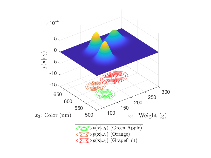
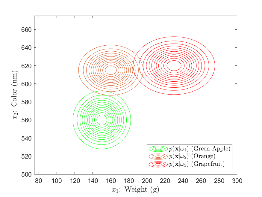
Here, we see that the likelihood distributions are Gaussian in shape, exhibiting the tell-tale “bell curve”. From these, we can gather a large amount of information about our classes. For example , we see that the green apple, orange, and grapefruit classes have approximately average weights of 150g, 160g, and 230g, respectively. With regards to color, this is associated with a mean wavelength of around 560nm, 615nm, and 620nm. Further, the orange and grapefruit classes exhibit a greater variance in weight as opposed to the apple class. Conversely, the apple and grapefruit classes seem to vary more widely in color than does the orange class.
However, most importantly, is the fact that these distributions represent the probability of observing a specific weight and color pair given that the fruit is either an apple, orange, or grapefruit. For example, consider the scenario in which the self-checkout measures the weight and color pair, 170g and 585nm. We can evaluate each likelihood distribution at ![\mathbf{x} = [170, 585]^{T}](https://ianmcatee.com/wp-content/ql-cache/quicklatex.com-05a4d58814cf024eeecda126c41b56f8_l3.png "Rendered by QuickLaTeX.com") to determine the probability of this observation given each class.
to determine the probability of this observation given each class.
Likelihood Calculations
Calculating the likelihood probability of a particular observation for each class involves evaluating the likelihood PDF at that observation. In our case, we have an observation of a fruit weighing 170g with a color wavelength of 570nm. We represent this as the two-dimensional feature vector:

Our likelihood distributions are of a multivariate Gaussian form,  , such that:
![\begin{equation*} p(\mathbf{x}|\omega_{j}) = \frac{1}{(2\pi)^{d/2}|\boldsymbol{\Sigma}_{j}|^{1/2}} \exp \left[-\frac{1}{2}(\mathbf{x}-\boldsymbol{\mu}_{j})^{t} \boldsymbol{\Sigma}_{j}^{-1} (\mathbf{x}-\boldsymbol{\mu}_{j})\right] \end{equation*}](https://ianmcatee.com/wp-content/ql-cache/quicklatex.com-fe0b0912d58c75d0faceee89b3328d4e_l3.png "Rendered by QuickLaTeX.com")
Here is the dimensionality of the feature vector . The Gaussian parameters  and
and  are the
  mean vector and
  covariance matrix for the jth class. In our case, the dimensionality is 2, and the Gaussian parameters have the form:

For our example fruit likelihoods, the mean vectors and covariance matrices for our three classes are given as:

Using these, the likelihood probability of our observation for each class can be calculated as follows:
Green Apple Likelihood:
![\begin{align*} p(\mathbf{x}|\omega_{1}) &= \frac{1}{(2\pi)|\boldsymbol{\Sigma}_{1}|^{1/2}} \exp \left[-\frac{1}{2}(\mathbf{x}-\boldsymbol{\mu}_{1})^{t} \boldsymbol{\Sigma}_{1}^{-1} (\mathbf{x}-\boldsymbol{\mu}_{1})\right]\\ \\ &= \boxed{6.1364 \times 10^{-5}} \end{align*}](https://ianmcatee.com/wp-content/ql-cache/quicklatex.com-0548a14b216298e95631683ed74efe6c_l3.png "Rendered by QuickLaTeX.com")
Orange Likelihood:
![\begin{align*} p(\mathbf{x}|\omega_{2}) &= \frac{1}{(2\pi)|\boldsymbol{\Sigma}_{2}|^{1/2}} \exp \left[-\frac{1}{2}(\mathbf{x}-\boldsymbol{\mu}_{2})^{t} \boldsymbol{\Sigma}_{2}^{-1} (\mathbf{x}-\boldsymbol{\mu}_{2})\right]\\ \\ &= \boxed{3.3501 \times 10^{-5}} \end{align*}](https://ianmcatee.com/wp-content/ql-cache/quicklatex.com-5e9d2a28c80e4b304324ad84dac27ac9_l3.png "Rendered by QuickLaTeX.com")
Grapefruit Likelihood:
![\begin{align*} p(\mathbf{x}|\omega_{3}) &= \frac{1}{(2\pi)|\boldsymbol{\Sigma}_{3}|^{1/2}} \exp \left[-\frac{1}{2}(\mathbf{x}-\boldsymbol{\mu}_{3})^{t} \boldsymbol{\Sigma}_{3}^{-1} (\mathbf{x}-\boldsymbol{\mu}_{3})\right]\\ \\ &= \boxed{2.9236 \times 10^{-7}} \end{align*}](https://ianmcatee.com/wp-content/ql-cache/quicklatex.com-48358e384a83664044a7eb125eecffb3_l3.png "Rendered by QuickLaTeX.com")
For our weight and color observation, the likelihoods evaluate to  ,
,  , and
, and  . We can interpret this as meaning that the probability is
  ,
,  , and
, and  that a green apple, orange, and grapefruit will weigh 170g and have a color measuring 585nm. These are extraordinarily small numbers, however, we can see that the probability of an green apple having this specific weight and color is higher than that of the other two classes. Here, it starts to become clear how useful the likelihoods can be in making a classification decision. Knowing the likelihoods only, if the self-checkout machine measured a piece of fruit at 170g and 585nm, logically we should predict that the fruit is an apple. We’ll see that additional information can help refine our prediction, but these likelihood distributions will still serve as our foundation.
The Prior
The other term in the numerator of Bayes’ theorem ,  , is the a priori (or prior) probability. This denotes prior knowledge of the class probabilities irrespective of any observations. That is, in the absence of any observational information, the prior represents the probability that a class will appear. The prior can be determined in a variety of ways. One common method is to estimate the priors using the class frequency from the training data, using the formula:
(5) 
Here,  is the total number of training data samples and
  is the number of training samples corresponding to class . As an example, say we had a training data set for two classes with a total of 1000 samples, containing 700 examples of class and 300 examples of class . Using this method, we could simply set the priors as
  and
and  . It should be noted that this method is only appropriate in situations in which your training data is actually representative of your class frequencies. For example, imagine you were fishing for salmon and sea bass. Assuming that you’ve documented enough fish and there were not biases in your fishing technique, you could use this method to reasonably estimate the prior probability that you would catch either fish. This is because your training data (i.e. the type and number of fish) is correlated to the actual populations salmon and sea bass.
However, reconsider our fruit example, how should we define the class priors? Here, the priors represent the probability that an individual will check out with a certain fruit, without us knowing any other information . The class frequency method outlined above doesn’t seem to make sense in this situation. For instance, say we had a a collection of weight/color training data consisting of 300 green apple examples, 200 orange examples, and 500 grapefruit examples. The above technique would set the priors at 0.3, 0.2, and 0.5 for the apple, orange, and grapefruit classes, respectively. These priors would imply that, in general, the customer is more likely to buy a grapefruit. Here we see the inconsistency, the probability of a customer buying a particular fruit has no correlation with the amount of training data we collected. In our case, we should consider different methods for setting the prior. For instance, we could examine past shopping data in an attempt to deduce how likely shoppers are to buy apple, oranges, or grapefruits. One could go as far as developing statistical models that include factors such as current price and stock, to set the prior probabilities. Or in the simplest case, one may assume equiprobable priors (a common technique), in which we assume that there is an equal prior probability for each class. This is all to illustrate the fact that setting the priors is highly problem specific, and there are additional methods to set the prior other than simply using the class frequency. It is quite important to consider the priors carefully because as we’ll see, the value of the prior will greatly impact Bayesian classifications.
The Evidence
The denominator term is the evidence, a PDF outlining how likely any particular feature vector is to occur in general. The evidence can be calculated from the likelihood and prior as:
(6) 
The evidence is perhaps the least important term in the context of Bayesian classification. It simply serves as a scaling factor such that the output posterior probability, , is a valid probability between 0 and 1. In fact, we’ll see later that the evidence is frequently omitted in Bayesian classification implementations.
The Posterior
Lastly, and perhaps most importantly, let’s revisit the term we touched upon earlier. This is known as the a posteriori probability, or simply the posterior. As noted, is the probability that the class is  given the feature vector has been measured. When stated in this way, it is immediately evident how the posterior could be directly used for classification. In fact, as the probability for which Bayes’ theorem solves for, the posterior is the core of Bayesian classification.
To illustrate the posterior’s importance and how it can it is used for classification, let’s continue with our fruit example. Suppose that we determined that the class priors are  ,
,  , and
, and  for the green apple, orange, and grapefruit classes, respectively. Now using these priors and the likelihood distributions given in Figures 2 and 3, we can use Bayes’ theorem to calculate the posterior probability for any given measured feature observation. Consider our earlier case in which the self-checkout machine reports a weight of 170g and a color wavelength of 585nm. Knowing the priors and likelihood probabilities, the calculation of the posterior probability for each class is straightforward:
Posterior Calculations
To calculate the posterior for each class, we apply Bayes’ theorem:

Where we have set the priors as:

We previously found the likelihood probability for each class at the feature vector ![\mathbf{x} = [155, 585]^{t}](https://ianmcatee.com/wp-content/ql-cache/quicklatex.com-99c1e35481263cb87536cf70078e64d5_l3.png "Rendered by QuickLaTeX.com") to be:
to be:

Lastly, we note that the evidence is the same for each posterior:

Now using Bayes’ theorem with our particular priors and likelihoods yields the posterior probability for each class:
Green Apple Posterior:

Orange Posterior:

Grapefruit Posterior:

In this example case, the posteriors evaluate to approximately 0.6459, 0.3526, and 0.0015 for the green apple, orange, and grapefruit classes, respectively. To help us interpret these results, let’s keep in mind that the posteriors reflect the probability that the fruit on the scale is a green apple, orange, or a grapefruit, given that the checkout machine measured a weight of 190g and the color at 585nm. This translates to a 64.59%, 35.26%, and a 0.15% chance that the unknown fruit is an apple, orange, or grapefruit. Here we see why the calculation of the posterior is so paramount to classification. Considering only the posterior probabilities, it is obvious that we should classify the fruit on the scale as an apple, as our calculations show that it is the most probable choice.
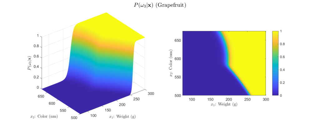
To get more intuition behind this, we can plot our example posteriors over a range of possible weight and color observations, as shown in Figures 4 to 6:
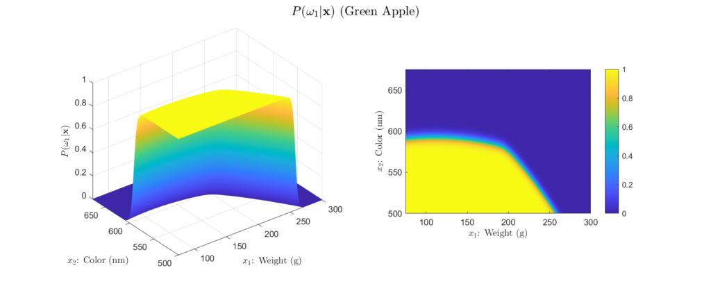

Left: Surface plot, Right: Heat map representation
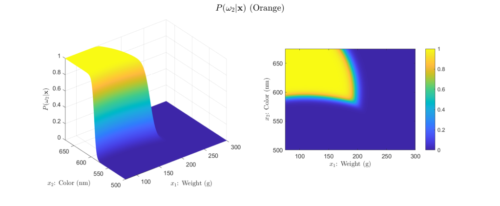

Left: Surface plot, Right: Heat map representation

Left: Surface plot, Right: Heat map representation
There are a few important aspects about the posteriors that these figures highlight. First, we see that the posteriors are all valid probabilities, meaning that the posteriors for all the classes sum to one for any observation. More importantly, these figures foreshadow the concept of decision regions. This is the idea that the feature space can subdivided into classification regions by maximum posterior. This results in a visual representation of how classifications will be assigned depending on the observation. We begin to see this in the heatmap representation of our example posteriors. Note how the yellow areas form a region in which, based only on the posteriors, we would classify as that class. This type of visualization is will prove very helpful for understanding why a Bayesian classifier makes the decisions it does. For example, consider Figure 5, we see that probability of the fruit being an orange becomes higher as the weight decreases and the color wavelength increases. This is logical, because oranges typically weigh less than grapefruit and their color is at a longer wavelength than that of a green apple. Decision regions will be discussed in more detail later, for now, it is interesting to note how the posterior plots relate to them.
We now see the foundation for how Bayes’ theorem can be used for classification. Fundamentally, we seek to calculate the posterior for each class and use the results to make a classification decision. As we’ll soon see, in many cases, the Bayesian decision rule for classification is exactly as described in our example, we simply choose the class associated with the highest posterior probability. However, there are other aspects that we can consider, and we’ll formalize Bayes’ decision rule in the next section.
Bayes’ Decision Rule
Thus far, we have heavily implied that the Bayes’ decision rule for classification involves predicting the class that coincides with the maximum posterior probability. However, while later we’ll show that this rule minimizes the probability of errors, it does not fully describe the cost associated with making certain classification decisions. Consider a situation in which you’ve made the wrong decision. Undoubtedly, there is a negative impact as result of your choice. However, there is a good chance that there were worse decisions, with harsher consequences. The same is true of classification problems. Sometimes misclassifying as a certain class is more costly than misclassifying as a different class.
Reconsidering our fruit example, suppose that the financial cost was $1, $2, and $3 for an apple, orange, and grapefruit respectively. Now, what if our system incorrectly classified a grapefruit as an apple or an orange and the customer was allowed to checkout? Both misclassifications result in a fiscal loss to the grocery store. However, misclassifying the grapefruit as an apple is more costly than misclassifying it as an orange, due to the greater price difference.
It is important to note that the costs of classification decisions can often be far more impactful than mere monetary loss. Suppose you have a classification system on a self-driving car. Now imagine the costs associated with misclassifying a stop sign as a tree, or worse, making the classification of “no pedestrian” when there is one. Either of these could result in physical harm. This example is to illustrate that misclassifications can have real-world impacts that need to be carefully considered.
Loss Functions
These types of misclassification costs can be accounted for in a loss function. The loss function  describes exactly how costly each action
  is, given that the class is . Note that in this context, an action could be making a classification or refusing to classify, known as a rejection. For notational simplicity, we can abbreviate the loss function as
  such that the loss function can be represented in matrix form:
(7) 
The loss function can sometimes be a point of confusion, therefore, let’s analyze it closer. Here we have an  number of possible actions, with each different action represented on each row of the loss matrix. Similarly, there are number of classes, as shown on the columns. In many simple cases, the only actions will be making classifications, that is, a rejection option isn’t considered in the loss function. Then,
  and the loss matrix is square, and we can interpret as loss when taking the action of predicting class i, when the true class is class j.
Consider this in the context of our fruit example. Recall that the green apple class is represented by , the orange class by , and the grapefruit class by As described earlier, suppose it costs $1 for an apple, $2 for an orange, and $3 for a grapefruit. One way of expressing our loss function would be:

Here we see that the diagonal elements are zero, because these represent correct classification decisions, and therefore, don’t have a cost. Conversely, the off-diagonals represent incorrect classifications and generally take non-negative positive values representing the magnitude of the corresponding loss. In situations in which all misclassifications are equally costly, it is common practice to set these losses as one. However, in our case, some misclassifications are literally more costly. We can see these losses encoded in elements  ,
,  , and
, and  , as these represent the cases in which a more expensive fruit is misclassified as a less expensive one. For example, is the loss incurred when an orange is misclassified as an apple. Because an orange is twice as expensive as the apple, we set this loss to 2. We can see this same logic in , and , the situations where a grapefruit is misclassified as an apple or an orange. A grapefruit is three times as expensive as an apple and two times as expensive as the orange, thus we set these elements to 3 and 2, respectively.
Risk
Further, we can find the expected loss of taking an action given our measurement of an input observation. Suppose that we observe some particular input feature vector and we decide to take the arbitrary action . Knowing that the posterior is the probability of the jth class and that we will incur a loss of if is the true class, then we can define the expected loss as:
(8) 
An expected loss is known as a risk, and  is the conditional risk. can be interpreted as the risk of taking action given that the feature vector has been observed. On closer inspection, one may begin to see how conditional risk can be used to form a general classification rule. We see that the conditional risk takes into account both the loss function and the Bayesian posterior probability to calculate the risk of any possible action. Intuitively, for a given input observation, we note that we could calculate the conditional risk for every possible action and then simply take the action corresponding to the least risk. In essence, this is the general Bayes’ decision rule.
General Bayes’ Decision Rule
Let’s formalize Bayes’ decision rule by showing that it is optimal in regards to risk. Note that an optimal decision rule would be one in which the overall risk was minimized by the chosen action. Let the decision rule be a function  such that one of an a number of actions
  is returned for each input . Then the overall risk
  is the expected (average) loss with regards to the decision rule as a whole given by:
(9) 
It is easy to see that the overall risk is minimized by minimizing the conditional risk  at every . This is equivalent to choosing such that is minimized. Thus we can state the general Bayes’ decision rule as:
(10) 
The minimum conditional risk found is known as the Bayes’ risk  . This represent the lowest risk possible and is associated with optimal classification with regards to overall risk.
To help clarify, let’s apply the general Bayes’ decision rule to our fruit example. As earlier, suppose that a weight of 170g and a color wavelength of 585nm were measured. Then using our previously calculated posterior probabilities and the loss matrix described earlier, we can find the conditional risk of making the green apple, orange, and grapefruit classification using equation (8):
Conditional Risk Calculations
Risk of Choosing Green Apple Class:

Risk of Choosing Orange Class:

Risk of Choosing Grapefruit Class:

Here, if we apply the general Bayes’ decision rule and take the action with the minimum conditional risk, we would choose action  and classify the fruit as an orange. This is an interesting result, as this classification is different than what we expected if we only looked at the posterior probability. Recall that the posterior probability was highest for the green apple class. Here we see how the incorporation of losses can affect the classification decision. Remember, we set the costs such that misclassifying an orange as an apple was twice as costly than the other way around. This potential loss overcame the high posterior probability that the fruit was an apple, and we classify as an orange instead. In general, the higher the loss is for a specific decision, the more risky that decision becomes, thus leading to a decreased chance overall that the action will be taken.
For our example, we can evaluate the conditional risk across a range of potential values. This allows us to use Bayes’ general decision rule to plot the decision regions for our classifier, as shown in Figure 7:
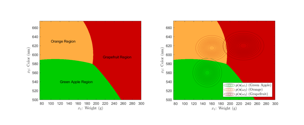
Left: Decision regions, Right: Decision regions with likelihood distributions superimposed
Here, we see the decision regions, or the regions of the feature space in which a particular classification decision will be made. This type of representation is helpful in understanding how Bayesian classifiers make decisions and how different aspects affect the final decision boundaries. For example, looking at the right plot of Figure 7, we see just how significant of an effect the likelihood distributions have on determining the final decision regions. Further, we can explore the influence that different loss functions can have on these boundaries. Imagine that there was an orange shortage, causing their price to rise significantly. To capture this new price difference, suppose we implemented the loss matrix:

Here we impose a steep penalty on misclassifying oranges as the other fruits. Using this loss matrix in our example classifier would yield decision regions as in Figure 8:
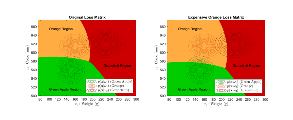
Left: Original loss function Right: Loss function that heavily penalizes misclassifying oranges
When comparing the decision regions that result from using the loss function that highly penalizes orange misclassification to that of our original decision regions, we see that the area corresponding to orange classification has greatly increased. This is a direct result of the associated high loss, as the classifier is more likely to classify the fruit as an orange in uncertain cases to avoid the potential misclassification penalty.
While we see see that losses have a significant impact, it is important to note that the posterior still is the fundamental value in Bayesian classification. The higher a class’s posterior probability is, the more likely it is to overcome the effect of potential losses. Regardless, one must carefully consider the loss function, as we see how drastically costs can affect the end classification decisions.
Minimum Error-Rate Classification
We have seen that the general Bayes’ decision rule provides for optimal classification with regards to overall risk. However, we noted how certain loss functions alter the risk and thus affect classification decisions. Unsymmetrical loss functions, such as that seen in our fruit example, can lead to more total classification errors, as the loss function effectively causes an overall shift toward less costly decisions. As discussed earlier, this is not necessarily a negative attribute, as there are many potential benefits to incorporating losses to certain decision. Nonetheless, there are many situations in which we seek to minimize the probability of error or error rate. This minimization can be accomplished by using the symmetrical, also known as the zero-one, loss function:
(11) 
The symmetry of this loss function is more evident if we examine it in its matrix form:
(12) 
As hinted by the name, the zero-one loss function does not penalize correct classifications and treats all misclassifications as equally costly by applying a unit loss. When represented as a matrix, zero-one loss function is square of dimensionality  , with possible actions corresponding to deciding one of the total classes. Correct decisions occur on the matrix diagonal where
  , with incorrect decisions on the off-diagonals. Using the zero-one loss function, the conditional risk can be simplified as:
(13) 
Note that this simplification takes advantage of the fact that all posterior probabilities must sum to one. Once again, we seek to minimize this conditional risk. It is straightforward to see that this minimization can be accomplished maximizing the posterior probability  . This is done by selecting the action that corresponds to the maximum posterior. Stated plainly, we simply decide the class that exhibits the maximum posterior probability for the given input observation . Formally, Bayes’ decision rule for minimum error rate can be expressed as:

Finally, we have justified the assumption made previously that the posterior probabilities alone can serve as a basis for classification. In fact, utilizing this simpler decision rule will yield optimal classification in terms of error rate. Meaning, that using the posteriors alone minimizes the average probability of errors, i.e. misclassifications. Further, because the posterior is the probability of class i given the specific observation , we can easily find the average probability of error as  . In no way does this mean that misclassifications will not occur, only that the classifier decisions are made in a way that minimizes the probability of errors.
Let’s once again return to our fruit example. Recall that for the measured weight and color pair, 170g and 585nm, we found the posteriors as  ,
,  , and
, and  . At the time, we merely postulated that based on the posterior values, we should classify the fruit as an apple. We now see that not only is this is valid classification decision, but utilizing only the posterior probabilities minimizes the probability of misclassifications. In this case, the probability of error is
  . This can be interpreted as there being an approximately 35.4% chance that the fruit is not an apple. As done earlier, we can use the minimum error rate form of Bayes’ decision rule to represent the decision regions of the classifier:

Left: Using minimum error rate Bayes’ decision rule, Right: Using general Bayes’ decision rule with a loss function
Here, we see the decision regions produced by the minimum error rate Bayes’ rule as opposed to the those produced by the general form. At first glance, they seem quite similar, however, a close examination shows slight differences in the decision regions. Recall that the general Bayes’ decision rule takes into account a loss matrix, while the minimum error rate form does not. We set the loss matrix such that misclassifications of more expensive fruit as less expensive fruit were penalized more. This results in a slight increase of the orange decision region area towards the apple region and similar increase of the grapefruit region towards the orange region, as compared to the regions described by the minimum error rate rule. As noted earlier, these changes in the decision boundaries serve to counterbalance the losses from costlier misclassifications.
These types of losses are not considered in the minimum error rate decision regions, as in that case, we assume all misclassifications are equally costly. The decision regions are only influenced by the likelihood distributions and the prior probabilities. We can see from the contours of the likelihood distributions in Figure 8, how their parameters shape help shape the decision regions.
However, we haven’t discussed how the prior probabilities affect the final decision regions. Recall that the prior probabilities represent the probability that the class will appear in general, that is, without having any observational data. We originally set our priors at 0.4, 0.4, and 0.2 for the green apple, orange, and grapefruit classes, respectfully. This indicates that the apple and orange classes have a higher probability to be bought on the whole than the grapefruit class. However, let’s explore the effects that different prior probabilities have on the decision regions:

While we don’t see any drastic changes, there are minute differences in the decision regions. In general, as you increase a class’s prior, you shift the decision boundaries towards the other classes means. That is, priors directly affect how large a decision region is for a particular class, with larger priors increasing the area of the decision region. We see this most clearly in the lower left plot of Figure 9, in which the green apple’s prior is 0.8. There, we see a distinct enlargement of the green apple decision region caused by this large prior. Because a large prior probability means that the class has a higher probability of occurring in general, it makes perfect sense that it would cause the resulting decision region to be overall larger. Even though the likelihoods distributions still play the dominant role in determining the relative size and shape of the decision regions, it is important to know how the prior probabilities contribute to the end classification decision boundaries.
While the minimum error rate form of Bayes’ decision rule is simple and convenient, it is important that you still consider other possible classification rules. While this form is well suited to many problems, it perhaps may only be a starting point for others. The incorporation of loss functions can help tailor the decision rule to your specific application. Moreover, there exists other loss functions, such as quadratic and linear-difference, and different Bayesian decision criteria, including minimax and Neyman-Pearson criterion. The discussion of such topics is beyond the scope of this article, however, it is recommended that one investigates such subjects prior to finalizing any Bayesian classifier, as they each address specific problems. In general, it will take careful consideration of the problem and most likely, substantial experimentation, before one finds the most effective Bayesian classification paradigm.
Bayesian Classifier Design
Knowing the basics of Bayesian decision theory, we now turn our focus to the functional structure of a Bayesian classifier. That is, how can we best organize the mathematics of Bayesian decision theory, such that we can perform classification efficiently? Firstly, it is helpful to visualize the structure of many classifiers as a network of functions, connecting the input observation and the final output classification decision. In the case of Bayesian classifiers, we often model the classifier as a discriminant function network, as shown in Figure 10:

As the name suggests, a discriminant function network utilizes a layer of discriminant functions to map the input observation to a classification action. In general, for a classifier with a number of output classes, there will be discriminant functions, each taking the d-dimensional feature vector as input. The discriminant functions also incorporate the potential costs, i.e. the loss function, into the classification action. A discriminant function network classifier assigns classifications based on the rule:
(14) 
Remember that each of the discriminant functions is associated with one of the possible classes. Therefore, this rule simply states that we choose the class associated with the discriminant function that yields the maximum output. Discriminant function networks are a general framework for describing many statistically-based classifiers. The discriminant functions essentially serve as a means to implement any given classification technique’s decision rule.
Bayesian Discriminant Functions
It is quite straightforward to adapt the Bayesian decision rule into the form of a discriminant function. Recall that in it’s most general form, the Bayes’ decision rule involves selecting the action such that the conditional risk is minimized. Thus we can write this general Bayes’ decision rule in the form of a discriminant function as:
(15) 
Here, we see that we can simply set each discriminant function to the negative of the conditional risk for a certain action. In this way, the maximum discriminant function will correspond to the minimum risk, thus reflecting the general Bayes’ decision rule. However, in the case of minimum error rate classification, i.e in situations with a zero-one loss function, we can simplify the discriminant function further to:
(16) 
Now each discriminant function represents the posterior probability of each class, and the classification is intuitively accomplished by choosing the class with the maximum posterior. Recall that the posterior is constrained between 0 and 1 as a probability. However, there is no need for this constraint in discriminant function networks. In fact, as long as the relative ordering between the outputs of the discriminant functions is preserved, the classification will remain accurate. Mathematically speaking, any monotonically increasing transformation can be applied to the discriminant function without any affect on classification. This property allows for forms of discriminant functions that simplify computations for different likelihood distributions. For example, for minimum error rate classification, both the following discriminant functions are valid and will yield the same classifications:
(17) 
(18) 
Here, the first equation is simply our original posterior probability discriminant function as calculated by Bayes’ rule. However, note that the evidence term is merely a scaling factor that ensures the posterior is a valid probability between 0 and 1. Eliminating this scaling will not affect the relative ordering of the discriminant outputs and thus we can safely ignore the evidence, resulting in the second equation. This is one of the most significant forms of the Bayesian discriminant function, as it is quite simple and can be used as a starting point for further optimization. Recall that the likelihood probability  may have the form of any probability distribution. Therefore, often times one will further refine the discriminant function to help simply calculations that arise from the specific PDF form of the likelihood.
Gaussian Discriminant Functions
In many cases, the likelihood density can be modeled as a Gaussian distribution. This is not unexpected, as Gaussian distributions are ubiquitous in statistics, with its familiar “bell curve” accurately describing the probability of many phenomenon. Because of its prevalence, Bayesian discriminant functions in the context of Gaussian likelihoods are well established. Commonly, in the Gaussian case, the following discriminant function is used:
(19) 
We arrive at this discriminant function by applying a natural logarithm to equation (18). This is valid because the natural logarithm is a monotonically increasing transformation, and as discussed, does not affect the relative ordering of discriminant outputs, thus preserving classification. At first, the introduction of the natural logarithm may seem to only add computational complexity to the discriminant function. However, if we examine this in the context of a Gaussian likelihood, we’ll see that this form will greatly simplify the discriminant calculation. First, let the ith class’s likelihood be a multivariate Gaussian distribution,  , such that:
(20) ![\begin{equation*} p(\mathbf{x}|\omega_{i}) = \frac{1}{(2\pi)^{d/2}|\boldsymbol{\Sigma}_{i}|^{1/2}} \exp \left[-\frac{1}{2}(\mathbf{x}-\boldsymbol{\mu}_{i})^{t} \boldsymbol{\Sigma}_{i}^{-1} (\mathbf{x}-\boldsymbol{\mu}_{i})\right] \end{equation*}](https://ianmcatee.com/wp-content/ql-cache/quicklatex.com-b2289df65a5ef694ae78c7257007553d_l3.png "Rendered by QuickLaTeX.com")
Here,  is the
  mean vector and
  is the covariance matrix , with being the input feature vector. Taking a closer look at this Gaussian form of the likelihood, one may see why it was beneficial to incorporate the natural logarithm into the discriminant function. By combining equations (19) and (20), the properties of logarithms allow us to express the discriminant as:
(21) ![\begin{equation*} \begin{split} g_{i}(\mathbf{x}) &= \ln \left(\frac{1}{(2\pi)^{d/2}|\boldsymbol{\Sigma}_{i}|^{1/2}} \exp \left[-\frac{1}{2}(\mathbf{x}-\boldsymbol{\mu}_{i})^{t} \boldsymbol{\Sigma}_{i}^{-1} (\mathbf{x}-\boldsymbol{\mu}_{i})\right]\right) + \ln P(\omega_{i}) \\ \\ &= -\frac{1}{2}(\mathbf{x}-\boldsymbol{\mu}_{i})^{t}\boldsymbol{\Sigma}_{i}^{-1}(\mathbf{x}-\boldsymbol{\mu}_{i}) - \frac{d}{2}\ln 2\pi - \frac{1}{2}\ln |\boldsymbol{\Sigma}_{i}| + \ln P(\omega_{i}) \end{split} \end{equation*}](https://ianmcatee.com/wp-content/ql-cache/quicklatex.com-35fff23985c115ff019de8cef0a299f4_l3.png "Rendered by QuickLaTeX.com")
Equation (21) Derivation
Rewrite the discriminant with the Gaussian likelihood:
![\begin{equation*} \begin{split} g_{i}(\mathbf{x}) &= \ln p(\mathbf{x}|\omega_{i}) + \ln P(\omega_{i}) \\ \\ &= \ln \left(\frac{1}{(2\pi)^{d/2}|\boldsymbol{\Sigma}_{i}|^{1/2}} \exp \left[-\frac{1}{2}(\mathbf{x}-\boldsymbol{\mu}_{i})^{t} \boldsymbol{\Sigma}_{i}^{-1} (\mathbf{x}-\boldsymbol{\mu}_{i})\right]\right) + \ln P(\omega_{i}) \end{split} \end{equation*}](https://ianmcatee.com/wp-content/ql-cache/quicklatex.com-f28fe5a26668fe68e673504d45f9cc7c_l3.png "Rendered by QuickLaTeX.com")
Use the product rule of logarithms to split the first term into a summation:
![\begin{equation*} g_{i}(\mathbf{x}) = \ln{\left( \frac{1}{(2\pi)^{d/2}|\boldsymbol{\Sigma_{i}}|^{1/2}}\right)} + \ln{\left( \exp{\left[-\frac{1}{2}(\mathbf{x} - \boldsymbol{\mu}_{i})^{t}\boldsymbol{\Sigma}_{i}^{-1}(\mathbf{x} - \boldsymbol{\mu}_{i}) \right]} \right)} + \ln P(\omega_{i}) \end{equation*}](https://ianmcatee.com/wp-content/ql-cache/quicklatex.com-a143d17604535f7ac1b4155dc8afd301_l3.png "Rendered by QuickLaTeX.com")
Using the quotient rule of logarithms, split the first fractional term into a subtraction. Noting the property,  , allows the elimination of the exponentiation in the second term, yielding:

Because  , the first term can be dropped. The second term can be split into a summation by the product rule of logarithms, giving:

Finally, using the power rule of logarithms to bring the exponents down in the first and second terms, and rearranging yields the discriminant as in equation (21):

We see that utilizing the natural logarithm has allowed us to eliminate the exponentiation present in the Gaussian likelihood. However, we can simplify further by noting term  is independent of the class. That is, it is a constant that does not affect classification in any way and can be dropped. This yields the general form of our Gaussian discriminant function:
(22) 
It is common to express this general Gaussian discriminant function in the form:
(23) 
Where,
(24) 
(25) 
(26) 
Equations (23-26) Derivation
Starting from equation (22), expand the quadratic term:

Distribute the 1/2 to the expanded quadratic term:

Let,

and

Then by substitution:

Noting that  is a symmetric square matrix, it can be said that
  is also symmetric. Further because the transpose of a symmetric matrix is identical to the original matrix, one notes that
  . Using this observation, it can be written:

Using the property of transposes,  , yields:

Lastly, letting,

and then substituting, gives the final form as in equation (23):

At first, expressing the discriminant like this may seem like pointless notational manipulation. However, in actual implementations of Bayesian classifiers, this form of the discriminant saves computations and improves efficiency. Let’s remember that matrix multiplication, and especially matrix inversion, are computationally complexity. Equation (26) allows for the pre-calculation and caching of several of the computational complex terms, thus lessening the computational burden when evaluating a new observation . This is beneficial from a efficiency standpoint and yields the same classification as the discriminant form in equation (22).
Parameter Estimation
As discussed, Bayesian classification relies on statistical knowledge of the problem, specifically, being able to describe the likelihood distributions  and prior probabilities . Unfortunately, in most problems, these statistics are not exactly known. Earlier, we covered different methods to estimate the prior probability, but never elaborated on the likelihood distributions. Given that the likelihoods are the major contributing factors in Bayesian classification, their estimation warrants a detailed explanation. Specifically, we’ll discuss parameter estimation. Parameter estimation encompasses a variety of techniques in which the form of a probability distribution can be reasonably assumed, and one must only estimate a set of parameters that describe the given distribution. For example, if we are confident that the likelihoods are Gaussian in form, then we merely have to find estimates for the mean and variance/covariance parameters. This estimate of the likelihood estimate distribution can now be used directly in the Bayesian discriminant function calculations.
Training Data
Typically, to estimate the likelihood distributions, we rely on our general knowledge of the problem as well as a set of observational samples known as the training data . Training data is a set of prerecorded observations that are representative of the classes. That is, each training data sample is a feature vector that has been measured from a known class. The class associated with each training data sample is often referred to as the label. Mathematically, for a classifier of classes, we will have sets of training data  with the samples in
  corresponding to the jth class .
Recall that the likelihood distribution represents the probability of observing specific feature vectors given a particular class. Therefore, theoretically, we can say that the training data for the jth class was drawn from the distribution . Because of this, we can use the training data to help describe the statistics of the likelihood . It is from this training data, that we’ll extract the statistical parameters (such as the mean and variance in the Gaussian case) of the likelihood distribution. However, it is important to give careful attention and consideration to your training data. The estimation of the likelihood distribution parameters can only be as good as the quality of the training data. Therefore, it is crucial that your training data actually be representative of your classes. That is, each training data sample should accurately reflect the features of the class it corresponds to. Further, we need enough training data to ensure that our parameter estimates are accurate. In parameter estimation, the estimates will converge on the true parameter values as the training data sample size increases (assuming representative data and correct model choice). There is no hard-and-fast rule on how much training data is required, as it is highly application dependent. In general, you should obtain as much quality training data as possible. However, there does exist a point of diminishing returns where additional data won’t noticeably improve estimates. A small training data sample size or non-representative training samples will lead to sub-optimal or plain incorrect parameter estimates, often referred to as estimate error, and will adversely affect classification performance.
As mentioned earlier, parameter estimation techniques require that you know the form of the likelihood distributions. While you may have a preliminary idea of the likelihood shape from the problem context, the training data can often provide direct evidence for the underlying distribution. For instance, you may assume that the likelihoods are Gaussian in form. By simply plotting the training data, a visual inspection can often be enough to confirm or deny this assumption. However, this is merely a heuristic test, if one needs a more robust validation of the distribution form, there exists statistical methods that can measure how well data fits a particular distribution. These methods are known broadly as Goodness-of-Fit tests, and although outside the scope of this article, may be helpful to research on your own.
Let’s return once again to our fruit example. In our case, the training data would consist of a collection of weight () and color ( ) measurements of numerous different green apples, oranges, and grapefruit such that:

Where  ,
,  , and
, and  are the training data sets consisting of a
  ,
,  , and
, and  number of examples for the green apple, orange, and grapefruit classes, respectively. Suppose that we had 1000 training data samples of each class, that is,
  . Because our training data is only two dimensional, we can easily get a sense the class distributions via a simple scatter plot:
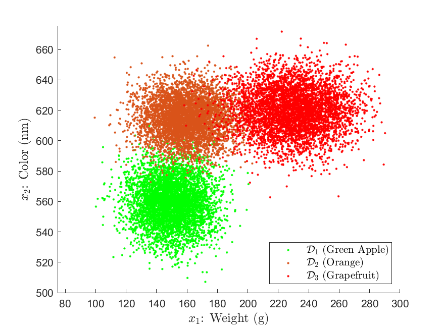
The clustering in Figure 11 offers compelling support that the underlying likelihood distributions of our training data are Gaussian in shape. We can also glean a sense of of the distribution parameters. For example, looking at the green apple training data, we can see that the mean is likely around  with a relatively spherical covariance. However, because we are fairly certain the distributions are Gaussian, we will see how we can use parameter estimation, and maximum likelihood estimation specifically, to obtain precise estimates of the means and covariances.
Maximum Likelihood Estimation
Maximum likelihood estimation (MLE) is a standard method of performing parameter estimation. MLE relies on the premise that the training data samples for the  class have been drawn from the likelihood distribution, and thus can be used to estimate the parameters of that distribution. That is, we assume that the samples of are independent identically distributed (i.i.d) random variables drawn from . Remember, in MLE, we know the form of the distribution , so we only seek the parameters of the distribution. In this context, parameters are the variables that describe a particular distribution. Each different type of probability distribution will have its own unique parameters. For example, in the Gaussian case, the parameters are the mean () and variance or covariance (
 or ). In contrast, a Gamma distribution has different parameters, namely a shape parameter (
 ) and a rate parameter (
 ). To generalize our MLE notation, we will denote the distribution parameters as a vector
  . Therefore, in the Gaussian case,
 ![\boldsymbol{\theta}_{j} = [\boldsymbol{\mu}_{j}, \boldsymbol{\Sigma}_{j}]^{t}](https://ianmcatee.com/wp-content/ql-cache/quicklatex.com-0c2d0cd4be963f3dc8e59ae9913252bc_l3.png "Rendered by QuickLaTeX.com") . To make it explicit that the likelihood distribution is parameterized by , we can write it as
. To make it explicit that the likelihood distribution is parameterized by , we can write it as  . This makes it obvious that the distribution depends not only on the class, but on its specific parameters. To simplify the notation, we can assume that each class’s training data is independent of one another, allowing us to drop the subscript and work with each class on its own. Therefore, going forward, we will simply write
  and
and  for the likelihood distribution and its associated training data, respectively. However, as we cover MLE, it is important to remember that there are still a number of likelihood distributions and training data subsets.
At its core, MLE seeks to estimate the parameter vector  of the distribution , given the training data . More plainly, we are trying to find parameters such that the distribution best reflects one that could have produced the training data. Suppose that the training data set has feature vector samples
  . Because each sample is assumed independent, we can write:
(27) 
Here,  represents the probability of observing the dataset given a particular set of parameters . Here, we can see that the best estimate for is one that maximizes the probability . Recall from our Bayes theory discussion, that the probability can be viewed as a likelihood in the context of a function of . Hence, the reason this technique known as maximum likelihood estimation.
For many types of distributions, it is often mathematically easier to work with the logarithm of the distribution. Because logarithms are a monotonically increasing transformations, maximization of the logarithm will yield the same result as maximizing the original function. Here, we take the natural logarithm of our parameter likelihood:
(28) 
(29) 
Our goal is to maximize  , known as the log-likelihood function, with respect to :
(30) 
Here,  is the estimate for the parameter vector that we seek, also known as the maximum likelihood estimator. Given that is differentiable in and meets the necessary conditions for the occurrence of a maximum, can be found via differential calculus based optimization. For such techniques, lets recall that the gradient operator with respect to the
  -element is defined as:
(31) 
From this definition, in conjunction with equation (30), we show that the gradient of the log likelihood function is:
(32) 
Because the gradient represents the direction of greatest change, function maxima must occur at points in which the gradient is zero. Therefore, to satisfy equation (30) and find our parameter estimate , we must solve the set of equations given by:
(33) 
For some forms of , equation (33) can be solved explicitly. However, there are models for which no closed form solution exists. In such cases, the parameter estimate may be found be numerical optimization techniques. Even in cases in which a solution to equation (30) can be found, the solution merely represents critical points of log likelihood . Recall that a critical point is any point in which the gradient is zero. At the function global maximum, the gradient is indeed zero, however, the gradient is also zero at the global minimum and all local maxima and minima. Therefore, it is important that we check each solution, either numerically or with a second derivative test, to find the solution that represents the global maximum.
It is important to remember that is still merely an estimate of the parameters of the likelihood distribution . The quality of the estimate is directly proportional to the amount of training data available. The reliability of the estimate decreases as the number of training data samples decrease. Only in the limit of an infinite sample size, does the estimate converge with the true parameter values.
Gaussian ML Estimation
In Bayesian classification, it is often the case that the likelihood can be modeled as a Gaussian distribution. Because of this, the details of Gaussian maximum likelihood estimation warrant its own discussion. Suppose that we have a univariate Gaussian distribution  and the training data set with samples
  . Here, the parameters are the mean and variance, as represented by
 ![\boldsymbol{\theta} = [\mu, \sigma]^{t}](https://ianmcatee.com/wp-content/ql-cache/quicklatex.com-7b7c4bf2eeca4bcb1a4b44d2e7872c16_l3.png "Rendered by QuickLaTeX.com") . Remember, we seek the estimates for the mean and covariance,
. Remember, we seek the estimates for the mean and covariance,  and
and  . Fortunately, in the Gaussian case, the application of the MLE method is well described and equation (33) results in a neat closed form solution:
(34) 
(35) 
This is a pleasing result, as those well-versed in statistics should immediately recognize these as the equations for sample mean and population variance. In fact, it is through MLE that we arrive at these common formulas. Similarly, in the case of multivariate Gaussian, where  and
and ![\boldsymbol{\theta} = [\boldsymbol{\mu}, \boldsymbol{\Sigma}]^{t}](https://ianmcatee.com/wp-content/ql-cache/quicklatex.com-4dbaf01f7faaf2702fd4b4036b49db5d_l3.png "Rendered by QuickLaTeX.com") , the maximum likelihood estimators can be found to be:
, the maximum likelihood estimators can be found to be:
(36) 
(37) 
Most texts on MLE include only a derivation of the univariate case. Because of this, coupled with the fact that the multivariate form is more general, I have included a full derivation of the multivariate Gaussian estimators below. While the derivation of the multivariate case is more involved than that of its univariate counterpart, I find that working through it is helpful for an understanding of the MLE process. Further, if you can successfully derive the multivariate case, the univariate form becomes trivial to find.
Equations (36-37) Derivation
First, we begin with the familiar multivariate Gaussian distribution:

The Gaussian is parameterized by two variables, the mean  and the covariance such that:

The probability of the data set given a particular parameterization is:
![\begin{align*} p(\mathcal{D}|\boldsymbol{\theta}) &= \prod_{k=1}^{n} p(\mathbf{x}_{k}|\boldsymbol{\theta}) \\ \\ &= \prod_{k=1}^{n} \left[ \frac{1}{(2\pi)^{d/2}|\boldsymbol{\Sigma}|^{1/2}} \exp \left(-\frac{1}{2}(\mathbf{x}_{k}-\boldsymbol{\mu})^{t} \boldsymbol{\Sigma}^{-1} (\mathbf{x}_{k}-\boldsymbol{\mu})\right) \right] \end{align*}](https://ianmcatee.com/wp-content/ql-cache/quicklatex.com-e93efbfe98dd535ab91e81af5890bfc2_l3.png "Rendered by QuickLaTeX.com")
Take the natural logarithm to obtain the log likelihood, note the details of taking the logarithm of the multivariate Gaussian were given earlier in the derivation of equation (21):
![\begin{align*} l(\boldsymbol{\theta}) &\equiv \ln p(\mathcal{D}|\boldsymbol{\theta}) \\ \\ &= \sum_{k=1}^{n}\ln{p(\mathbf{x}_{k}|\boldsymbol{\theta)}} \\ \\ & = \sum_{k=1}^{n} \ln \left[ \frac{1}{(2\pi)^{d/2}|\boldsymbol{\Sigma}|^{1/2}} \exp \left(-\frac{1}{2}(\mathbf{x}_{k}-\boldsymbol{\mu})^{t} \boldsymbol{\Sigma}^{-1} (\mathbf{x}_{k}-\boldsymbol{\mu})\right) \right] \\ \\ &= \sum_{k=1}^{n} - \frac{d}{2}\ln 2\pi - \frac{1}{2}\ln |\boldsymbol{\Sigma}| -\frac{1}{2}(\mathbf{x}_{k}-\boldsymbol{\mu})^{t}\boldsymbol{\Sigma}^{-1}(\mathbf{x}_{k}-\boldsymbol{\mu}) \\ \\ &= - \frac{nd}{2}\ln 2\pi - \frac{n}{2}\ln |\boldsymbol{\Sigma}| - \frac{1}{2} \sum_{k=1}^{n} (\mathbf{x}_{k}-\boldsymbol{\mu})^{t}\boldsymbol{\Sigma}^{-1}(\mathbf{x}_{k}-\boldsymbol{\mu}) \end{align*}](https://ianmcatee.com/wp-content/ql-cache/quicklatex.com-a5dc5a0c48d261a483e240eb25fb5f15_l3.png "Rendered by QuickLaTeX.com")
Take the gradient of the log-likelihood function and set it equal to zero:

This leads to a system of two equations that must be solved:

Lets first examine the partial derivative  :
:
![\begin{equation*} \frac{\partial l}{\partial \boldsymbol{\mu}} = \frac{\partial}{\partial \boldsymbol{\mu}} \left[ - \frac{nd}{2}\ln 2\pi - \frac{n}{2}\ln |\boldsymbol{\Sigma}| - \frac{1}{2} \sum_{k=1}^{n} (\mathbf{x}_{k}-\boldsymbol{\mu})^{t}\boldsymbol{\Sigma}^{-1}(\mathbf{x}_{k}-\boldsymbol{\mu}) \right] \end{equation*}](https://ianmcatee.com/wp-content/ql-cache/quicklatex.com-8f7493acf374d8eba63b031e2ed82658_l3.png "Rendered by QuickLaTeX.com")
We can safely ignore any terms without a , as these evaluate to zero when taking the partial derivative:
![\begin{equation*} \frac{\partial l}{\partial \boldsymbol{\mu}} = -\frac{1}{2} \sum_{k=1}^{n} \frac{\partial}{\partial \boldsymbol{\mu}} \left[ (\mathbf{x}_{k}-\boldsymbol{\mu})^{t}\boldsymbol{\Sigma}^{-1}(\mathbf{x}_{k}-\boldsymbol{\mu}) \right] \end{equation*}](https://ianmcatee.com/wp-content/ql-cache/quicklatex.com-15e4007c06b79ade0c6ed13d2a6f68bd_l3.png "Rendered by QuickLaTeX.com")
To simplify, we first note the identity  ([4], eq. 86), allowing us to write:

Now set the expression to zero and solve for :

Left multiply each side by to eliminate the term:

Use the properties of summations to bring the out of the summation:

From here, basic algebraic manipulation allows us to find our mean estimator  :
:

Now we contend with the partial derivative with respect to the covariance,  :
:
![\begin{equation*} \frac{\partial l}{\partial \boldsymbol{\Sigma}} = \frac{\partial}{\partial \boldsymbol{\Sigma}} \left[ - \frac{nd}{2}\ln 2\pi - \frac{n}{2}\ln |\boldsymbol{\Sigma}| - \frac{1}{2} \sum_{k=1}^{n} (\mathbf{x}_{k}-\boldsymbol{\mu})^{t}\boldsymbol{\Sigma}^{-1}(\mathbf{x}_{k}-\boldsymbol{\mu}) \right] \end{equation*}](https://ianmcatee.com/wp-content/ql-cache/quicklatex.com-35790b59cd5f28087e494cb3843c7b3d_l3.png "Rendered by QuickLaTeX.com")
Once again, we ignore any terms without :
![\begin{align*} \frac{\partial l}{\partial \boldsymbol{\Sigma}} &= \frac{\partial}{\partial \boldsymbol{\Sigma}} \left[- \frac{n}{2}\ln |\boldsymbol{\Sigma}|\right] - \frac{\partial}{\partial \boldsymbol{\Sigma}} \left[\frac{1}{2} \sum_{k=1}^{n} (\mathbf{x}_{k}-\boldsymbol{\mu})^{t}\boldsymbol{\Sigma}^{-1}(\mathbf{x}_{k}-\boldsymbol{\mu}) \right] \\ \\ &= - \frac{n}{2}\frac{\partial}{\partial \boldsymbol{\Sigma}}\left[\ln |\boldsymbol{\Sigma}|\right] -\frac{1}{2}\sum_{k=1}^{n} \frac{\partial}{\partial \boldsymbol{\Sigma}} \left[ (\mathbf{x}_{k}-\boldsymbol{\mu})^{t}\boldsymbol{\Sigma}^{-1}(\mathbf{x}_{k}-\boldsymbol{\mu}) \right] \end{align*}](https://ianmcatee.com/wp-content/ql-cache/quicklatex.com-0d3b56eaf3b8b2a906985abd679c5879_l3.png "Rendered by QuickLaTeX.com")
Here we have two terms to differentiate with respect to . Lets first approach the ![\frac{\partial}{\partial \boldsymbol{\Sigma}} \left[\ln |\boldsymbol{\Sigma}|\right]](https://ianmcatee.com/wp-content/ql-cache/quicklatex.com-51d69eac47a4aeeba9b8fabf91193952_l3.png "Rendered by QuickLaTeX.com") term. Here we use the identity
term. Here we use the identity  ([4], eq. 57). This allows us to write:
![\begin{equation*} \frac{\partial l}{\partial \boldsymbol{\Sigma}} =-\frac{n}{2}(\boldsymbol{\Sigma}^{-1})^{t} - \frac{1}{2}\sum_{k=1}^{n} \frac{\partial}{\partial \boldsymbol{\Sigma}} \left[ (\mathbf{x}_{k}-\boldsymbol{\mu})^{t}\boldsymbol{\Sigma}^{-1}(\mathbf{x}_{k}-\boldsymbol{\mu}) \right] \end{equation*}](https://ianmcatee.com/wp-content/ql-cache/quicklatex.com-3f7869af4ffcc129c7c47fd2e23a9721_l3.png "Rendered by QuickLaTeX.com")
Because is a square symmetric matrix,  , therefore:
![\begin{equation*} \frac{\partial l}{\partial \boldsymbol{\Sigma}} =-\frac{n}{2}\boldsymbol{\Sigma}^{-1} - \frac{1}{2}\sum_{k=1}^{n} \frac{\partial}{\partial \boldsymbol{\Sigma}} \left[ (\mathbf{x}_{k}-\boldsymbol{\mu})^{t}\boldsymbol{\Sigma}^{-1}(\mathbf{x}_{k}-\boldsymbol{\mu}) \right] \end{equation*}](https://ianmcatee.com/wp-content/ql-cache/quicklatex.com-3f3b734749395d406271f2bd073824b3_l3.png "Rendered by QuickLaTeX.com")
For the ![\frac{\partial}{\partial \boldsymbol{\Sigma}} \left[ (\mathbf{x}{k}-\boldsymbol{\mu})^{t}\boldsymbol{\Sigma}^{-1}(\mathbf{x}{k}-\boldsymbol{\mu}) \right]](https://ianmcatee.com/wp-content/ql-cache/quicklatex.com-df56329aa1eeea3bda44048549902459_l3.png "Rendered by QuickLaTeX.com") term, we use the identity
term, we use the identity  ([4], eq. 61):

Once again using the fact that , we have:

Set  to zero and solve for :

To get the ML estimator  , we need to solve for . First take the inverse of both sides of the expression:

To simplify this further, we need to note the inverse matrix properties  and
and  . Using these, we can write:

Right multiply both sides by :

Here,  is the identity matrix. Finally, solve for by right multiplying by
  and dividing by :

To illustrate how Gaussian MLE works, let’s return one last time to our fruit example. With the green apple, orange, and grapefruit training data (, , and ), we can apply equations (36) and (37) to obtain the following parameters:

Here, we see our estimated means  and covariance matrices
  that correspond to our fruit class’s likelihood distributions
  . We can plot these distributions to get a better idea how the estimated likelihoods fit the training data:
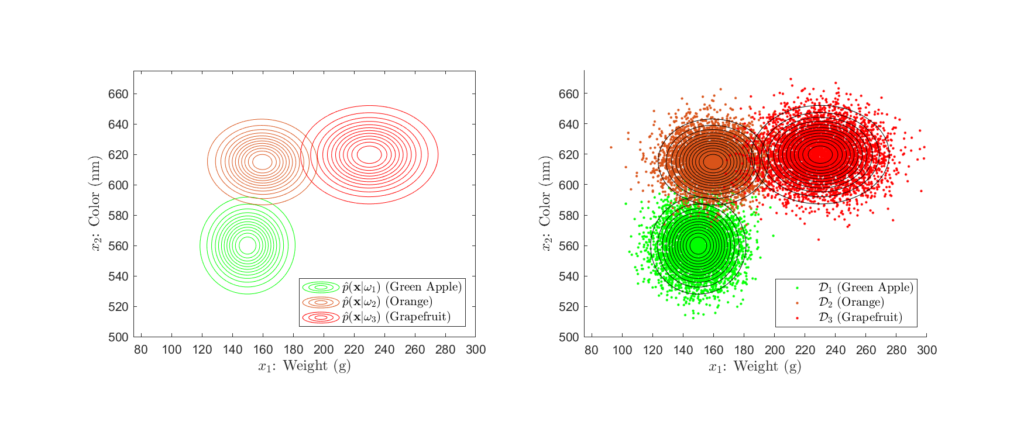
Left: Contour plot only, Right: Contour plot superimposed on training data
Figure 12 shows that the estimated likelihood distributions fit the training data quite well. But how can we tell exactly how accurate the maximum likelihood estimators were? For full disclosure, our sample green apple, orange, and grapefruit training data is synthetic data. Because of this, we know the actual distributions that the training data samples were drawn from. Therefore, we can directly compare the estimated parameters to the true parameters:

Comparing the true means and covariances ( ) and their associated maximum liklihood estimates (
 ), we see that they are very close. Indeed, if we plot the the true and estimated likelihood distributions next to one another, we’d be hard-pressed to tell a difference:
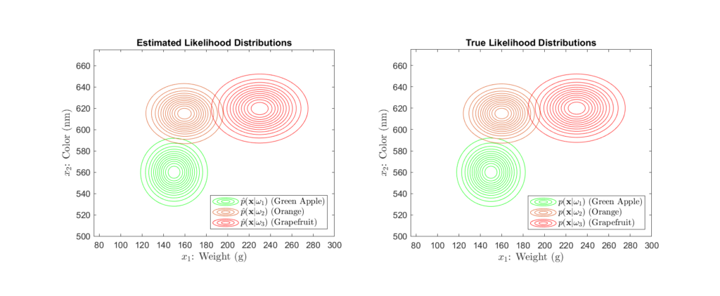
Left: MLE estimated distributions, Right: True distributions from which the training data was drawn
From Figure 13, it is clear that our estimated likelihood distributions closely approximate their true counterparts. Now we see why parameter estimation techniques are commonly used to obtain the estimates of the likelihood distributions for Bayesian classification. Under the right circumstances, these techniques offer quite accurate parameter estimations and given enough training data, even converge to the true parameter values. Although, it is important to stress that this example demonstrates ideal circumstances. Our example data was cleanly drawn from known distributions. Training data in real-world applications is often not truly independent and can suffer from artifacts such noise. Thoughtful data collection and preprocessing techniques are often required to form a training data set suitable for MLE. However, if one is able to acquire a quality training dataset, that is representative of the classes, parameter estimation techniques can easily help approximate likelihood distributions to form the basis for Bayesian classification.
Python Implementation
Here, we will adapt our mathematical Bayesian classification framework into Python code. For continuity sake, we will use the same fruit classification example that we have developed thus far. First, we develop a Python class to serve as a container for the Bayesian classification process. Then we will write some driver code to implement this Bayesian classification class with some artificial data that statistically matches our apple, orange, and grapefruit example.
Bayesian Classifier Class
First we implement a Python class that will allow us to train our Bayesian classifier and classify new data:
### BAYESIAN CLASSIFIER CLASS ###

# Import Numpy to work with arrays
import numpy as np

'''
Class: BayesianClassifier
Description:
   Class to implement Bayesian classification
Inputs:
   trainingData: Multiple DxN numpy arrays containing the training data
   for each class, where D is the number of features and N is the number
   training examples. Note this class assumes Gaussian training data
   priors: (Optional) A list of floats of the same length as the number of
   classes, must sum to one. If no priors provided, equiprobable priors will
   be used
'''
class BayesianClassifier:
  def __init__(self, *trainingData, priors = []):
    # Check if the training data is present for at least two classes
    if not trainingData : raise Exception("No Training Data Provided")
    if len(trainingData) < 2:
      raise Exception("Must Provide Training Data For More Than One Class")

    # Define private class variables
    self.numClasses = 0
    self.numFeatures = 0
    self.priors = []
    self.estimatedMeans = []
    self.estimatedCovs = []
    self.W = []
    self.w = []
    self.w0 = []

    # Check if the input is valid, initialize private variables
    self.__CheckAndInitializeData(trainingData, priors)

    # Estimate the data statistics
    self.__EstimateDataStatistics(trainingData)
    self.__Train(trainingData)

  # Private method to check the training data and priors format and
  # initialize private variables
  def __CheckAndInitializeData(self, trainingData, priors):

    # Check the training data format
    numFeat = trainingData[0].shape[0]
    for data in trainingData:
      if type(data) is not np.ndarray:
        raise Exception("Training data must be NumPy array")
      if len(data.shape) > 2:
        raise Exception("Training data must be a DxN array")
      if data.shape[0] > data.shape[1]:
        raise Exception("Number of training samples must be greater "\
                        "than the number of features")
      if data.shape[0] != numFeat:
        raise Exception("Number of features not consistent across "\
                        "training data")
      numFeat = data.shape[0]

    # Set the number of classes and features
    self.numClasses = len(trainingData)
    self.numFeatures = numFeat

    # Check the priors format
    if priors:
      if type(priors) is not list:
        raise Exception("Priors must be of type list")
      if len(priors) != self.numClasses:
        raise Exception("Number of priors must match number of classes")
      if sum(priors) > 1.01 or sum(priors) < 0.99:
        raise Exception("Priors must sum to 1")
      self.priors = priors
    else:
      print("No priors provided, using equiprobable priors")
      self.priors = [1/self.numClasses]*self.numClasses

  # Private method to use Maximum Likelihood Estimation to estimate the
  # training data statistics
  def __EstimateDataStatistics(self,trainingData):

    # Iterate through training datasets
    for data in trainingData:
      # Get the number of samples in the current training data size
      n = data.shape[1]
      # Estimate data mean using eq.(34)
      mean = np.sum(data, axis = 1, keepdims=True)/n
      # Estimate data covariance eq.(35)
      s = np.zeros([self.numFeatures,self.numFeatures])
      for k in range(n):
        xVec = data[:,k]
        xVec.shape = (self.numFeatures, 1)
        xMinusMean = xVec - mean
        s += (xMinusMean).dot(xMinusMean.T)
      cov = s/n

      # Set the private variables for estimated mean and covariances
      self.estimatedMeans.append(mean)
      self.estimatedCovs.append(cov)

  # Private method to train the bayesian classifier by calculating the
  # discriminant terms
  def __Train(self,trainingData):

    #Calculate discriminant function terms
    for cls in range(self.numClasses):
      mean = self.estimatedMeans[cls]
      cov = self.estimatedCovs[cls]
      covInv = np.linalg.inv(cov)
      prior = self.priors[cls]
      self.W.append(-0.5*covInv) # eq.(24)
      self.w.append(covInv.dot(mean)) # eq.(25)
      self.w0.append(-0.5*(((mean.T).dot(covInv)).dot(mean)) \
                     -0.5*np.log(np.linalg.det(cov)) + np.log(prior)) # eq. (26)

    # Print the classifier parameters my invoking __str__
    print(self)

  # Public method to evaluate data using the trained classifier
  # Note, can evaluate a single x or an array of x values
  def Evaluate(self, x):

    # Check that input is a numpy array with the correct number of features
    if type(x) is not np.ndarray:
      raise Exception("Evaluation data must be of type numpy array")
    if x.shape[0] != self.numFeatures:
      raise Exception(\
          "Evalulation data must have {} features".format(self.numFeatures))

    # Check if input is a single data point, if so, reshape into a vector
    if len(x.shape) == 1:
      x.shape = (self.numFeatures,1)

    # Allocate the discrimant (g) and classification arrays
    g = []
    classification = []

    # Perform the classification by iterating through inputs
    for i in range(x.shape[1]):
      g = []
      xVec = x[:,i]
      # Calculate the discriminant function for each class
      for cls in range(self.numClasses):
        disc = (xVec.T.dot(self.W[cls])).dot(xVec) + self.w[cls].T.dot(xVec) \
                + self.w0[cls] # eq.(23)
        g.append(disc[0])
      #Classify by getting the max of the discriminant functions
      classification.append(g.index(max(g)) + 1)

    # Return the classification array
    return classification

  # Special method to print of the Bayesian classifier parameters
  def __str__(self):
    classStr = ""
    meanStr = ""
    covStr = ""
    priorStr = ""
    WStr = ""
    wStr = ""
    w0Str = ""
    for i in range(self.numClasses):
      classStr = "\tClass " + str(i+1) + ":\n"
      meanStr += classStr
      covStr += classStr
      priorStr += classStr + "\t\t" + str(self.priors[i]) + "\n"
      WStr += classStr
      wStr += classStr
      w0Str += classStr + "\t\t" + str(self.w0[i][0]) + "\n"

      for j in range(self.numFeatures):
        meanStr += "\t\t" + str(self.estimatedMeans[i][j]) + "\n"
        covStr += "\t\t" + str(self.estimatedCovs[i][j]) + "\n"
        WStr += "\t\t" + str(self.W[i][j]) + "\n"
        wStr += "\t\t" + str(self.w[i][j]) + "\n"

    outString = ("*********************************************\n"
              "BAYESIAN CLASSIFIER:\n"
              "Number of Classes: {}".format(self.numClasses) + "\n"
              "Number of Features: {}".format(self.numFeatures) + "\n"
              "\n-----------------------------------\n"
              "DATA STATISTICS:\n"
              "Estimated Means: \n {}".format(meanStr) + "\n"
              "Estimated Covariances: \n {}".format(covStr) + "\n"
              "Prior Probabilities: \n {}".format(priorStr) + "\n"
              "-----------------------------------\n"
              "BAYESIAN DISCRIMINANT VARIABLES:\n"
              "W: \n {}".format(WStr) + "\n"
              "w: \n {}".format(wStr) + "\n"
              "w0: \n {}".format(w0Str) + "\n"
              "*********************************************\n")
    return outString
This class has three important methods that warrant closer inspection. Let’s first look at the __EstimateDataStatistics method. This method implements maximum likelihood estimation on each class’s training data by applying the equations (36-37) to estimate the means and covariances. The __Train method then uses these estimations to calculate the discriminant function variables for each class, as outlined in equations (24-26). At this point, we consider our Bayesian classifier trained and can now use the EvaluateData method to classify new data. The EvaluateData method takes new data as input, calculates the discriminant function from equation (23), then assigns a classification based on the maximum discriminant.
The remainder of the code is simply boilerplate methods to ensure the training data and priors are of the correct format and to print the classifier parameters in a user-readable format.
Driver Code
Below is example driver code that implements our Bayesian classifier class:
### EXAMPLE DRIVER CODE ###

#Import libraries
import numpy as np
import matplotlib.pyplot as plt
from tabulate import tabulate

### GENERATE TRAINING DATA ###

#Define training data statistics
#Note these are only used to create our artificial multivariate data
appleMean = np.array([150, 560])
orangeMean = np.array([160, 615])
grapefruitMean = np.array([230,620])
appleCov = np.array([[200,0],[0,200]])
orangeCov = np.array([[250,0],[0,150]])
grapefruitCov = np.array([[400,0],[0,200]])

#Generate 1000 samples of multivariate random training data for each class
#Note these will be 2x1000 arrays
appleTrain = np.random.multivariate_normal(appleMean,appleCov,1000).T
orangeTrain = np.random.multivariate_normal(orangeMean,orangeCov,1000).T
grapefruitTrain = np.random.multivariate_normal(grapefruitMean,\
                                                grapefruitCov,1000).T
appleTest = np.random.multivariate_normal(appleMean,appleCov,1000).T
orangeTest = np.random.multivariate_normal(orangeMean,orangeCov,1000).T
grapefruitTest = np.random.multivariate_normal(grapefruitMean,\
                                               grapefruitCov,1000).T

#Plot the training data for visual inspection
x = plt.scatter(appleTrain[0,:],appleTrain[1,:], c = "green", marker='.', \
                label='Apple')
plt.scatter(orangeTrain[0,:],orangeTrain[1,:], c = "orange", marker='.', \
            label='Orange')
plt.scatter(grapefruitTrain[0,:],grapefruitTrain[1,:], c = "red", marker='.', \
            label='Grapefruit')
plt.title("Artificial Training Data")
plt.xlabel("x1 Weight (g)")
plt.ylabel("x2 Color (nm)")
plt.legend(loc='lower right')
plt.show()

### BAYESIAN CLASSIFICATION ###

# Define our prior probabilities
priorProbs = [0.4,0.4,0.2]

# Create an instance of our Bayesian classifier class
classifier = BayesianClassifier(appleTest,orangeTest,grapefruitTest, \
                                priors = priorProbs)

# Perform the Bayesian classification on the artificial test data
appleClassifications = classifier.Evaluate(appleTest)
orangeClassifications = classifier.Evaluate(orangeTest)
grapefruitClassifications = classifier.Evaluate(grapefruitTest)
classifications = [appleClassifications,orangeClassifications, \
                   grapefruitClassifications]

# Calculate the class and overall accuracy of the classifications
accuracies = []
errors = []
numMisclassifications = []
for i in range (3):
  unique, counts = np.unique(classifications[i], return_counts=True)
  numCorrect = counts[np.where(unique == i+1)[0][0]]
  numMisclassifications.append(1000-numCorrect)
  accuracies.append(numCorrect/1000)
  errors.append(1-accuracies[i])
overallError = sum(numMisclassifications)/3000
overallAccuracy = 1-overallError

# Form a table of the classifier accuracy and error percentages
accuracyTable = [
    ["", "Accuracy (%)","Error (%)"],
    ["Apple Class", accuracies[0]*100, errors[0]*100],
    ["Orange Class", accuracies[1]*100, errors[1]*100],
    ["Grapefruit Class", accuracies[2]*100, errors[2]*100],
    ["Overall", overallAccuracy*100, overallError*100]]

# Show a table of the classifier performance
print('CLASSIFIER ACCURACY (BY CLASS AND OVERALL):')
print(tabulate(accuracyTable, headers='firstrow', tablefmt='fancy_grid'))
Output:
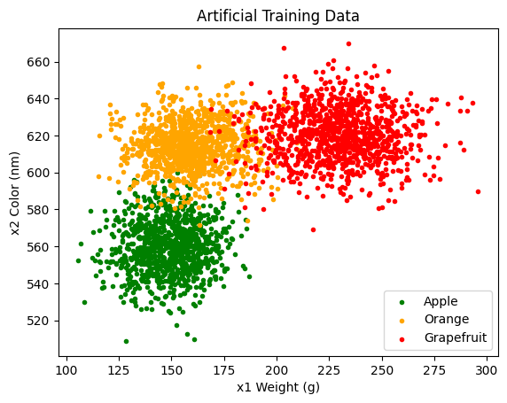
*********************************************
BAYESIAN CLASSIFIER:
Number of Classes: 3
Number of Features: 2

-----------------------------------
DATA STATISTICS:
Estimated Means:
 	Class 1:
		[150.37973903]
		[560.89604937]
	Class 2:
		[159.35012433]
		[614.69751562]
	Class 3:
		[230.0805077]
		[619.66884803]

Estimated Covariances:
 	Class 1:
		[183.4614201   0.7174097]
		[  0.7174097  202.94687409]
	Class 2:
		[252.52231456  -1.79687041]
		[ -1.79687041 141.14576154]
	Class 3:
		[413.33749814   6.07561807]
		[  6.07561807 207.31687782]

Prior Probabilities:
 	Class 1:
		0.4
	Class 2:
		0.4
	Class 3:
		0.2

-----------------------------------
BAYESIAN DISCRIMINANT VARIABLES:
W:
 	Class 1:
		[-2.72540631e-03  9.63421064e-06]
		[ 9.63421064e-06 -2.46373300e-03]
	Class 2:
		[-1.98020242e-03 -2.52091674e-05]
		[-2.52091674e-05 -3.54275815e-03]
	Class 3:
		[-1.21018654e-03  3.54656663e-05]
		[ 3.54656663e-05 -2.41280633e-03]

w:
 	Class 1:
		[0.8088842]
		[2.76089864]
	Class 2:
		[0.66208303]
		[4.36348344]
	Class 3:
		[0.51292673]
		[2.97396193]

w0:
 	Class 1:
		[-841.28722445]
	Class 2:
		[-1400.01961304]
	Class 3:
		[-987.73148023]

*********************************************

CLASSIFIER ACCURACY (BY CLASS AND OVERALL):
╒══════════════════╤════════════════╤═════════════╕
│                  │   Accuracy (%) │   Error (%) │
╞══════════════════╪════════════════╪═════════════╡
│ Apple Class      │           98.5 │         1.5 │
├──────────────────┼────────────────┼─────────────┤
│ Orange Class     │           97.7 │         2.3 │
├──────────────────┼────────────────┼─────────────┤
│ Grapefruit Class │           96.3 │         3.7 │
├──────────────────┼────────────────┼─────────────┤
│ Overall          │           97.5 │         2.5 │
╘══════════════════╧════════════════╧═════════════╛
Here, we first create some artificial training and test data that matches our apple, orange, and grapefruit example by sampling multivariate Gaussians with the same defined statistics. We then scatter plot our training data to visually confirm that it appears Gaussian with the proper means and variances.
In the next section of code, we define our prior probabilities and use our training data to instantiate an instance of Bayesian classifier class. Successful instantiation of the Bayesian classifier results in the estimated training data statistics and calculated Bayesian discriminant function variables being printed to the console. The trained classifier is then used to perform the classification of our artificial test data by calling its Evaluate method. This results in arrays of labels that denote the predicted class for each test data sample. Because we know the correct classification for the test data, we calculate and display the accuracy and error of our classifier for each class and overall.
Analysis
If we examine our classification results, we see that our Bayesian classifier performs quite well, with an overall accuracy of 97 .5%. From our theoretical discussion of Bayesian classification and the well-discriminable Gaussian data, this is to be expected. As mentioned earlier, from a statistical perspective, our classifier exhibits optimal performance with regards to error minimizations. This, paired with the fact that our artificial data was drawn from actual Gaussian distributions and our maximum likelihood estimations closely resemble the actual statistics, explains our classifier’s high performance. However, it is important to keep in mind that our example is purely artificial. In a real-world implementation, it is doubtful that the training data would be as well-behaved and much consideration would have to be paid to its measurement and preprocessing. Nonetheless, the basic process as shown in our example will serve as a solid foundation and starting point for most problems in which Bayesian classification is well suited.
Final Thoughts
Bayesian classification is a foundational technique in machine learning and provides a statistical basis for many other algorithms. Recently, it seems like we have become inundated in new and trendy artificial intelligence technologies. However, among these advancements, it is important that we not forget about more elementary machine learning techniques. There exists applications in which the state-of-the-art AI networks aren’t warranted. For simple problems, one may save computational complexity and achieve similar results by using basic statistical methods. Further, in some fields, medical, military, or transportation for example, we need to know the certainty associated with classification decisions. This is something modern “black-box” AI tools struggle with determining. While these systems are often highly accurate, it is difficult to assess how these decisions were reached and how confident we can be in them. On the contrary, risk calculations are integral to statistical classification methods, such as Bayesian classification. The ability to mathematically support the certainty of a decision is beneficial in high risk applications. Further, Bayesian classifier exhibit statistical decision optimality that other techniques are simply unable to surpass. In closing, as we move forward, and AI becomes more integrated into our lives, it is important that we are selecting the proper methodologies and architectures on a problem-by-problem basis, and not based on current tech fads.
References
[1] R. O. Duda, P. E. Hart, and D. G. Stork, Pattern Classification, 2nd ed. John Wiley & Sons Inc., 2001.
[2] C. W. Therrien and M. Tummala, Probability and Random Processes for Electrical and Computer Engineers, 2nd ed. CRC Press, 2012.
[3] D. C. Lay, S. R. Lay, and J. J. McDonald, Linear Algebra and Its Applications, 5th ed. Upper Saddle River, NJ: Pearson Education Inc, 2016.
[4] K. B. Petersen and M. S. Pedersen, The Matrix Cookbook. Kongens Lyngby, DK: Technical University of Denmark, 2012.