Tutorial GitHub: https://github.com/IanMcAtee/NIfTI-To-Image-Sequence
What is a NIfTI file?
A NIfTI file is common file type used to store volumetric medical imaging data. Specifically, NIfTI primarily encodes data from neuroimaging scans, such as those from MRI, CT, and others. The manufacturers of medical scanners (Phillips, Siemens, GE, etc.) usually have their own proprietary data storage formats. Therefore, the Neuroimaging Informatics Technology Initiative developed the aptly named NIfTI file to serve as a standardized way to store and distribute these neuroimaging scans. NIfTI files are easily recognizable from their .nii extension or its compressed .nii.gz extension.
What are we trying to accomplish?
Most radiological image viewing software can open and view NIfTI format scans. However, there may be occasions in which you want the scan’s slices in a standard image format, for example, PNG or JPEG. This could be for a variety of purposes, such as for easier display, for image processing, or for use in a machine learning dataset. However, simple tools to extract the NIfTI scan views as images seem few and inadequate. Therefore, here, we’ll use Python and open-source libraries to perform this image conversion manually.
Extracting image sequences from NIfTI Scan
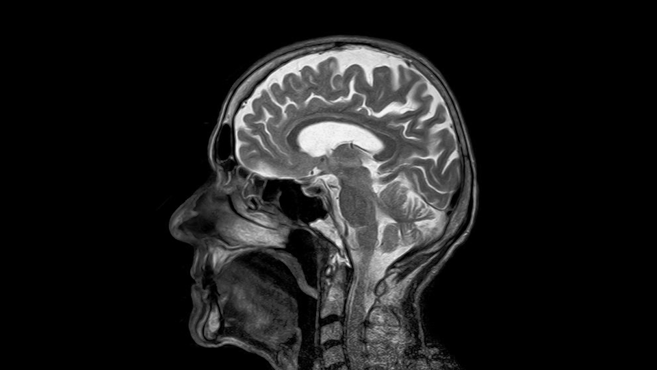
Here, we’ll go over a step-by-step of how to extract and save an image sequence for each of the views from a NIfTI file. As an example, I’ll be using an brain MRI that I sourced from the 3D Slicer software. This NIfTI file will also be available at the GitHub for this tutorial.
Step 1: Install NiBabel and other necessary libraries
In order to access and manipulate NIfTI scans in Python, we’ll need a specialized library. For this tutorial, we’ll be using NiBabel, however, there are many other libraries that can open and manipulate NIfTI data. NiBabel is a low-level Python library that gives access to a variety of imaging formats, including NIfTI, with a particular focus on providing a common toolkit to the various volumetric formats produced by scanners. You can find more information about NiBabel as well as its API documentation at https://nipy.org/nibabel/.
You can install NiBabel from your Python terminal. If you use PIP, you can install NiBabel with the following command:
pip install nibabel
Alternatively, you can install NiBabel with Conda by using:
conda install -c conda-forge nibabel
You’ll also need to have the following common packages installed:
- Numpy (https://numpy.org/)
- Matplotlib (https://matplotlib.org/)
- OpenCV (https://opencv.org/)
If you don’t already have these packages installed, visit their associated links for installation instructions.
Step 2: Create a new Python script and import libraries
To start, open a new Python script in your code editor of choice. Personally, I prefer Jupyter notebook and the notebook I used in this tutorial will be available on the GitHub, as linked at the top of this post. First off, let’s import all the necessary libraries at the top of our script:
#Import necessary libraries
import nibabel as nib
import matplotlib.pyplot as plt
import numpy as np
import cv2
Step 3: Use NiBabel to extract and examine the NIfTI scan data
Here, we’ll use NiBabel to load our NIfTI scan and extract its data array. I’ll also present a introductory explanation of some of the important properties of NIfTI scans and we’ll view a few image slices.
Load the NiFTI scan and extract the scan’s data array
The first step in working with any NIfTI scan with NiBabel is to load the scan. This is usually followed by extracting the scan’s data array, that is, the multidimensional array that actually contains the volumetric image data. To do this, we’ll use the following code:
#Define the filepath to your NIfTI scan
scanFilePath = 'c:/Users/Desktop/MRHead.nii'

#Load the scan and extract data using nibabel
scan = nib.load(scanFilePath)
scanArray = scan.get_fdata()
Examining this code, we see that we first specify a variable scanFilePath to hold the file path to your NIfTI file. For simplicity, we are simply using a string to hold this path, however, feel free to use the common os.path method for this if you wish. To load a NIfTI image in NiBabel, we use the .load method and assign it to a scan variable. This returns an NiBabel object of the NiFTI scan and allows us to view and modify some properties of the scan. To get the actual multidimensional array that contains the values of the volumetric image, we use the .get_fdata() method. We assign this to the scanArray variable which will usually result in either a three or four dimensional array depending on the type of scan. In our example case, the MRI scan will be represented as a three dimensional array for the x, y, and z spatial dimensions. In the case that your scan is a volumetric time series, you will get a four dimensional array with the extra dimension denoting the time axis.
Like any array, we can examine the shape of the data array via the .shape property. Using the following, let’s save the shape of the data array to a scanArrayShape variable and print the shape to the console:
#Get and print the scan's shape
scanArrayShape = scanArray.shape
print('The scan data array has the shape: ', scanArrayShape)
For our example MRI scan, this prints the following to the console:
The scan data array has the shape: (256, 256, 130)
We can see that our scan array has a dimensionality of 256x256x130. Because an MRI is a volumetric scan, each of the elements in this array represent a voxel (volumetric pixel) produced by the scanner. We can view this three dimensional array from three different perspectives, thus yielding two dimensional images of the axial, coronal, and sagittal anatomical planes. That is, we have 130 image slices that are 256×256 and two sets of 256 slices that are 256×130.
Before continuing, it is important to note that unless otherwise specified, dimensionality in this tutorial is referred to in common matrix notation. That is, an array of 256×130 has 256 rows with 130 columns. Thus an image produced from this array will have a width of 130 and a height of 256. Keep this in mind as we discuss the data array moving forward.
Examine the NIfTI scan properties via the header
All NIfTI scans have an associated header. The header is metadata that contains a variety of information about the scan. Let’s print out the NIfTI header for closer examination using the .header property:
#Examine scan's shape and header
scanHeader = scan.header
print('The scan header is as follows: \n', scanHeader)
For our example, running this will result in the following output:
The scan header is as follows:
 <class 'nibabel.nifti1.Nifti1Header'> object, endian='<'
sizeof_hdr      : 348
data_type       : b''
db_name         : b''
extents         : 0
session_error   : 0
regular         : b'r'
dim_info        : 0
dim             : [  3 256 256 130   1   1   1   1]
intent_p1       : 0.0
intent_p2       : 0.0
intent_p3       : 0.0
intent_code     : none
datatype        : int16
bitpix          : 16
slice_start     : 0
pixdim          : [1.        1.        1.        1.2999954 0.        0.        0.
 0.       ]
vox_offset      : 0.0
scl_slope       : nan
scl_inter       : nan
slice_end       : 0
slice_code      : unknown
xyzt_units      : 2
cal_max         : 0.0
cal_min         : 0.0
slice_duration  : 0.0
toffset         : 0.0
glmax           : 0
glmin           : 0
descrip         : b''
aux_file        : b''
qform_code      : scanner
sform_code      : scanner
quatern_b       : -0.5
quatern_c       : 0.5
quatern_d       : -0.5
qoffset_x       : -86.6449
qoffset_y       : 133.9286
qoffset_z       : 116.7857
srow_x          : [ -0.          0.          1.2999954 -86.6449   ]
srow_y          : [ -1.      -0.      -0.     133.9286]
srow_z          : [  0.      -1.       0.     116.7857]
intent_name     : b''
magic           : b'n+1'
We can see that a NIfTI header contains quite a bit of information about the scan. An explanation of all these header fields is beyond the scope of this tutorial. However, if you are curious, Anderson Winkler gives an excellent description of all the NIfTI header fields in his article at https://brainder.org/2012/09/23/the-nifti-file-format/.
For our purposes, we need to pay attention to the pixDim field of the header. This field describes the physical dimensions of the voxels in the scan’s data array. That is, the size of the voxels in the world space. The values at indexes 1, 2, and 3 in the pixDim field correspond to the voxel dimensions in the x, y, and z axis, respectively. If we examine our example MRI scan’s header, we can see that these indexes of the pixDim field (pixDim[1:4]) are [1, 1, 1.2999954]. Hence, we can deduce that the voxel dimensions in our scan are approximately 1x1x1.3. The units of the voxel dimensions can be extrapolated from the xyzt_units field of the header. In our case, this value is 2, indicating that the units used are in millimeters.
View the middle scan slice along each dimension
Before proceeding, we should take a moment to view a few of the scan images to ensure they are what we expect. Using the following code, we can display the middle image slice along each of our scan array’s dimensions:
#Display scan array's middle slices
fig, axs = plt.subplots(1,3)
fig.suptitle('Scan Array (Middle Slices)')
axs[0].imshow(scanArray[scanArrayShape[0]//2,:,:], cmap='gray')
axs[1].imshow(scanArray[:,scanArrayShape[1]//2,:], cmap='gray')
axs[2].imshow(scanArray[:,:,scanArrayShape[2]//2], cmap='gray')
fig.tight_layout()
plt.show()
For our MRI, this produces the following figure:
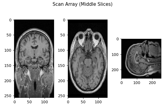
As expected, we see the coronal, axial, and sagittal slices of a head MRI depicted in the first, second, and third images, respectively. However, upon close inspection, the axial and coronal slices appear to exhibit a slight vertical stretching. The reason for this is related to the voxel dimensions discussed earlier and the default way MatPlotLib’s imshow function displays images. Recall that the voxel dimensions in our MRI scan were approximately 1x1x1.3. Therefore, for true anatomical perspective, when viewing a slice in the coronal and axial planes, the pixels need to have a width of 1.3 and a height of 1. However, MatPlotLib’s imshow function will display arrays with standard square pixels. When displaying information that was originally intended to have a pixel width of 1.3 and height of 1 as a square pixel, this results in an apparent shrinking of the image along the horizontal axis, thus yielding a stretched perspective.
View the middle scan slices with anatomical aspect ratio
To view a more anatomically accurate form of the scan’s axial and coronal slices, we can adjust the aspect ratio of the images. Fortunately, the imshow function has an aspect parameter, allowing us to set a custom aspect ratio. However, we first must determine the aspect ratio that aligns with the proper anatomical dimensions. Recall that aspect ratio is defined as:
![\[ r =\frac{w}{h} \]](https://ianmcatee.com/wp-content/ql-cache/quicklatex.com-4c49b801018856ae7c14fcd7a35aaa9d_l3.png "Rendered by QuickLaTeX.com")
Where r is the aspect ratio, and w and h are the image width and height, respectively. Because of our voxel dimensions, in the axial and coronal views, the width should be 1.3 with a height of 1. However, because pixels rendered on a display must always be square, we can write:
![\[ 1.3w = h \]](https://ianmcatee.com/wp-content/ql-cache/quicklatex.com-cd0091da9ee91bf67a26ac9b67351299_l3.png "Rendered by QuickLaTeX.com")
That is, for every one unit of height, there needs to be 1.3 units of width. Solving this for aspect ratio yields:
![\[ r = \frac{w}{h} = \frac{1}{1.3} \approx 0.77 \]](https://ianmcatee.com/wp-content/ql-cache/quicklatex.com-13476b6f7b1b2e65f84a3285056f2018_l3.png "Rendered by QuickLaTeX.com")
In Python, we use the previous formulas to calculate the proper aspect ratio for each of the anatomical views as follows:
#Calculate proper aspect ratios
pixDim = scanHeader['pixdim'][1:4]
aspectRatios = [pixDim[1]/pixDim[2],pixDim[0]/pixDim[2],pixDim[0]/pixDim[1]]
print('The required aspect ratios are: ', aspectRatios)
Which will produce the output:
The required aspect ratios are: [0.76923347, 0.76923347, 1.0]
As we can see, this produces the correct aspect ratios for each of the anatomical views. That is, approximately 0.77 for the axial and coronal views and 1 for the sagittal view, as it already was in the proper aspect ratio. We can modify the code used previously for displaying the middle scan slices to account for these proper aspect ratios by implementing the aspect parameter in the imshow function as follows:
#Display scan array's middle slices with proper aspect ratio
fig, axs = plt.subplots(1,3)
fig.suptitle('Scan Array w/ Proper Aspect Ratio (Middle Slices)')
axs[0].imshow(scanArray[scanArrayShape[0]//2,:,:], aspect = aspectRatios[0], cmap='gray')
axs[1].imshow(scanArray[:,scanArrayShape[1]//2,:], aspect = aspectRatios[1], cmap='gray')
axs[2].imshow(scanArray[:,:,scanArrayShape[2]//2], aspect = aspectRatios[2], cmap='gray')
fig.tight_layout()
plt.show()
Thus producing the figure:
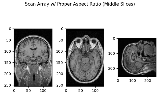
Comparing this figure to the previous, we can see that by using the voxel dimensions to account for the proper aspect ratio, the images slices do not exhibit stretching effects and appear to be in proper anatomical perspective. Unfortunately, using MatPlotLib, there is no way to bulk save these images with this proper aspect ratio. Therefore, the next sections will outline how to resample these image slice arrays such that their shape reflects this proper aspect ratio.
Step 4: Resample scan array and save as images
Calculate proper output scan array dimensions
In the last section, we detailed why one usually can not save the scan’s data array directly as images due to issues with the aspect ratio. Here, we’ll solve this by resampling the scan array slices to the proper aspect ratio prior to saving. To do this, we need to calculate new dimensions for each scan view such to reflect an anatomical aspect ratio. Once again, this can be done by looking at the scan’s voxel dimensions. Recall our scan array had a shape of 256x256x130 with a voxel dimensionality of 1x1x1.3. As we have seen, the sagittal slices do not require any resampling as the they already have a uniform pixel size of 1×1. Recall that earlier we stated that because of the voxel dimensions, for anatomical perspective in the axial and coronal views, the width needs to be 1.3 times as large as the height. In our example, a slice of the scan array in the axial and coronal views is 256×130. Remember, that this is in array dimensionality, meaning that its width is 130 and the height is 256. Therefore, for anatomical perspective we must resample these slices to a width of 169, i.e 130 * 1.3, with the same height of 256. To find these new array dimensions for each scan view, we use the following code:
#Calculate new image dimensions from aspect ratio
newScanDims = np.multiply(scanArrayShape, pixDim)
newScanDims = (round(newScanDims[0]),round(newScanDims[1]),round(newScanDims[2]))
print('The new scan dimensions are: ', newScanDims)
For our example, this will output:
The new dimensions are: (256, 256, 169)
By examining the code, you can see that to arrive at the new scan dimensions for resampling, we simply do an element-wise multiplication of the scan array shape and the voxel dimensions, remembering to round to ensure whole numbers. As expected, from the output we see that the sagittal slices need to be saved as arrays of 256×256, while the axial and coronal slices as arrays of 256×130.
Resample and save the scan array slices as images
To resample and save the scan array as images, we’ll be using the popular computer vision and image processing library OpenCV. Specifically, we’ll use the resize function to resample the axial and coronal slices and the imwrite function to save the arrays as images. The code we use to accomplish this is listed below, followed by a explanation of its operation:
#Set the output file path
outputPath = 'c:/Users/Desktop/MR_Head_Images'

#Iterate and save scan slices along 0th dimension
for i in range(scanArrayShape[0]):
    #Resample the slice
    outputArray = cv2.resize(scanArray[i,:,:], (newScanDims[2],newScanDims[1]))
    #Save the slice as .png image
    cv2.imwrite(outputPath+'/Dim0_Slice'+str(i)+'.png', outputArray)

#Iterate and save scan slices along 1st dimension
for i in range(scanArrayShape[1]):
    #Resample the slice
    outputArray = cv2.resize(scanArray[:,i,:], (newScanDims[2],newScanDims[0]))
    #Save the slice as .png image
    cv2.imwrite(outputPath+'/Dim1_Slice'+str(i)+'.png', outputArray)

#Iterate and save scan slices along 2nd dimension
for i in range(scanArrayShape[2]):
    #Resample the slice
    outputArray = cv2.resize(scanArray[:,:,i], (newScanDims[1],newScanDims[0]))
    #Rotate slice clockwise 90 degrees
    outputArray = cv2.rotate(outputArray, cv2.ROTATE_90_CLOCKWISE)
    #Save the slice as .png image
    cv2.imwrite(outputPath+'/Dim2_Slice'+str(i)+'.png', outputArray)
To resample and save the scan’s data array as images, we first start be defining the file path to an output directory, i.e the folder you want to contain all of the slice images. We assign this output file path string to an outputPath variable. We then iterate through each of the scan data array’s dimensions and use the imwrite function to save each array slice as a .png image to the output file path. Note that the first parameter in the imwrite function is the full output path of the saved image, which we form by appending the output path variable with a unique image file name with the suffix .png. In the case of the axial and coronal views (dimensions 0 and 1), prior to saving, we use the resize function to resample them to 256×130. Here, the first parameter of the resize function is the array to be saved and the second parameter is a tuple in the form (width, height) that we create from the newScanDims variable calculated earlier. Also, recall that when we viewed the sagittal slice, it appeared rotated counterclockwise by 90 degrees. Therefore, we used OpenCV’s rotate function to rotate the slice clockwise by 90 degrees prior to saving. Depending on your specific scan, you may need to implement rotation on other dimensions as well.
If we run this code and check the output directory, we should see all of the slices of our scan saved as .png images that reflect the proper anatomical aspect ratio:
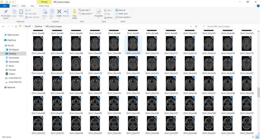
And with that, we have all the slices of the NIfTI scan as .png images. You can now use these image as you see fit like any other image file.
An important note on resampling
Here, we resampled the axial and coronal slices such that they reflected the actual anatomical aspect ratio. It is very important to note that OpenCV’s resize function uses interpolation to achieve this. Interpolation always involves the creation of new pixel values that were not present in the original data. This new pixel creation can be accomplished with various mathematical methods that consider the pixels values around the locations of the new pixels. Specifically, by default, the resize function uses a method known as bilinear interpolation. Therefore, while these slices are visually accurate with regards to aspect ratio, to achieve this meant the introduction of new pixel data into the image. For most applications, this minor introduction of new data is not an issue. However, if your purposes require absolute data accuracy, you might consider not resampling or may want to look more deeply into how the resampling is performed.
Final Thoughts
Over the last half century, volumetric scans such a MRI and CT have revolutionized healthcare by providing spatial imaging capabilities to clinicians. Now, thanks to file format such NIfTI and open source tools like NiBabel, the examination and manipulation of this type of data is easier than ever. In this tutorial, we simply extracted the scan view slices as individual images. However, hopefully through this tutorial, you came to realize that this only merely begins to touch upon the type of manipulations you can perform on NIfTI scans. From machine learning techniques for automated pathology recognition, to medical image guided surgical robotics, their basis can be found in working with these types of medical image formats and their associated data arrays. I hope that this tutorial is but a beginning step on your journey to implementing a new technology based on this type of medical data.
Until next time,
Ian McAtee
Full Code
For reference, the full code used in this tutorial is listed below:
#Import necessary libraries
import nibabel as nib
import matplotlib.pyplot as plt
import numpy as np
import cv2

#Define the filepath to your NIfTI scan
scanFilePath = 'c:/<YOUR NIFTI FILE PATH>'

#Load the scan and extract data using nibabel
scan = nib.load(scanFilePath)
scanArray = scan.get_fdata()

#Get and print the scan's shape
scanArrayShape = scanArray.shape
print('The scan data array has the shape: ', scanArrayShape)

#Get and print the scan's header
scanHeader = scan.header
print('The scan header is as follows: \n', scanHeader)

#Display scan array's middle slices
fig, axs = plt.subplots(1,3)
fig.suptitle('Scan Array (Middle Slices)')
axs[0].imshow(scanArray[scanArrayShape[0]//2,:,:], cmap='gray')
axs[1].imshow(scanArray[:,scanArrayShape[1]//2,:], cmap='gray')
axs[2].imshow(scanArray[:,:,scanArrayShape[2]//2], cmap='gray')
fig.tight_layout()
plt.show()

#Calculate proper aspect ratios
pixDim = scanHeader['pixdim'][1:4]
aspectRatios = [pixDim[1]/pixDim[2],pixDim[0]/pixDim[2],pixDim[0]/pixDim[1]]
print('The required aspect ratios are: ', aspectRatios)

#Display scan array's middle slices with proper aspect ratio
fig, axs = plt.subplots(1,3)
fig.suptitle('Scan Array w/ Proper Aspect Ratio (Middle Slices)')
axs[0].imshow(scanArray[scanArrayShape[0]//2,:,:], aspect = aspectRatios[0], cmap='gray')
axs[1].imshow(scanArray[:,scanArrayShape[1]//2,:], aspect = aspectRatios[1], cmap='gray')
axs[2].imshow(scanArray[:,:,scanArrayShape[2]//2], aspect = aspectRatios[2], cmap='gray')
fig.tight_layout()
plt.show()

#Calculate new image dimensions from aspect ratio
newScanDims = np.multiply(scanArrayShape, pixDim)
newScanDims = (round(newScanDims[0]),round(newScanDims[1]),round(newScanDims[2]))
print('The new scan size is: ', newScanDims)

#Set the output file path
outputPath = 'c:/<YOUR OUTPUT FILE PATH>'

#Iterate and save scan slices along 0th dimension
for i in range(scanArrayShape[0]):
    #Resample the slice
    outputArray = cv2.resize(scanArray[i,:,:], (newScanDims[2],newScanDims[1]))
    #Save the slice as .png image
    cv2.imwrite(outputPath+'/Dim0_Slice'+str(i)+'.png', outputArray)

#Iterate and save scan slices along 1st dimension
for i in range(scanArrayShape[1]):
    #Resample the slice
    outputArray = cv2.resize(scanArray[:,i,:], (newScanDims[2],newScanDims[0]))
    #Save the slice as .png image
    cv2.imwrite(outputPath+'/Dim1_Slice'+str(i)+'.png', outputArray)

#Iterate and save scan slices along 2nd dimension
for i in range(scanArrayShape[2]):
    #Resample the slice
    outputArray = cv2.resize(scanArray[:,:,i], (newScanDims[1],newScanDims[0]))
    #Rotate slice clockwise 90 degrees
    outputArray = cv2.rotate(outputArray, cv2.ROTATE_90_CLOCKWISE)
    #Save the slice as .png image
    cv2.imwrite(outputPath+'/Dim2_Slice'+str(i)+'.png', outputArray)